𝑖=1 𝑛∑ λ𝑖* 𝑦𝑖 = 0
● 𝑥𝑖,𝑥𝑗 𝑑𝑎𝑡𝑎 𝑝𝑜𝑖𝑛𝑡𝑠 𝑦𝑖,𝑦𝑗 𝑐𝑙𝑎𝑠𝑠𝑒𝑠 𝑏𝑜𝑡ℎ 𝑎𝑟𝑒 𝑎𝑣𝑎𝑖𝑙𝑎𝑏𝑙𝑒 𝑖𝑛 𝑎 𝑑𝑎𝑡𝑎
▪ 𝑏𝑦 𝑎𝑝𝑝𝑙𝑦𝑖𝑛𝑔 𝑎𝑙𝑙 𝑜𝑢𝑟 𝑑𝑎𝑡𝑎 𝑝𝑜𝑖𝑛𝑡𝑠 𝑤𝑒 𝑐𝑎𝑛 𝑔𝑒𝑡 λ𝑖
▪ 𝑓𝑜𝑟 𝑒𝑎𝑐ℎ 𝑑𝑎𝑡𝑎 𝑝𝑜𝑖𝑛𝑡 𝑤𝑒 𝑤𝑖𝑙𝑙 𝑔𝑒𝑡 λ
𝑇ℎ𝑒 𝑔𝑜𝑎𝑙 𝑖𝑠 𝑛𝑜𝑤 𝑡𝑜 𝑓𝑖𝑛𝑑 𝑡ℎ𝑒 𝑜𝑝𝑡𝑖𝑚𝑎𝑙 λ
𝑇ℎ𝑒 λ𝑖 𝑣𝑎𝑙𝑢𝑒𝑠 𝑑𝑒𝑡𝑒𝑟𝑚𝑖𝑛𝑒 𝑤ℎ𝑖𝑐ℎ 𝑑𝑎𝑡𝑎 𝑝𝑜𝑖𝑛𝑡𝑠 𝑎𝑟𝑒 𝑠𝑢𝑝𝑝𝑜𝑟𝑡 𝑣𝑒𝑐𝑡𝑜𝑟𝑠 𝑖. 𝑒 λ 𝑖> 0 𝑗=1 𝑛 ∑ 𝑗=1 𝑛∑ λ ( 𝑖 , 𝑦 , j) (𝑥𝑖* 𝑥 𝑗) 𝑤12 +𝑤22 = ||𝑤|| = (𝑊 * 𝑊)12 =12 𝑤 * 𝑤𝐿(𝑥, 𝑦, λ) =12 𝑤 * 𝑤 − λ * 𝑦 * 𝑤𝑜 + 𝑤𝑇( 𝑥)
𝑆𝑡𝑒𝑝 − 1: 𝑀𝑎𝑘𝑒 𝑡ℎ𝑒 𝑐𝑙𝑎𝑠𝑠𝑒𝑠 𝑒𝑞𝑢𝑎𝑡𝑖𝑜𝑛 𝑦 𝑤𝑜 + 𝑤𝑇( * 𝑥) > 1𝑦 = 1
𝑐𝑙𝑎𝑠𝑠1 𝑒𝑞𝑢𝑎𝑡𝑖𝑜𝑛 𝑤𝑜 + 𝑤𝑇* 𝑥 > 1𝑦 =− 1
𝑐𝑙𝑎𝑠𝑠2 𝑒𝑞𝑢𝑎𝑡𝑖𝑜𝑛 𝑤𝑜 + 𝑤𝑇* 𝑥 < 1 𝑆𝑡𝑒𝑝 − 2: 𝐼𝑛𝑐𝑟𝑒𝑎𝑠𝑒 𝑡ℎ𝑒 𝑚𝑎𝑟𝑔𝑖𝑛 𝑑𝑖𝑠𝑡𝑎𝑛𝑐𝑒 𝑜𝑓 𝑡ℎ𝑒 𝑑𝑎𝑡𝑎 𝑝𝑜𝑖𝑛𝑡 𝑡𝑜 𝑡ℎ𝑒 ℎ𝑦𝑝𝑒𝑟𝑝𝑙𝑎𝑛𝑒 𝑑 =𝑤1 𝑥1+𝑤 2𝑦1+𝑤𝑜 | | 𝑤 12+𝑤 22 =𝑤1𝑥 1+𝑤 2𝑦1+𝑤𝑜 | | ||𝑊|| =𝑤𝑜+𝑤𝑇𝑥 ||𝑊|| 𝑆𝑡𝑒𝑝 − 3: 𝐷𝑒𝑐𝑟𝑒𝑎𝑠𝑒 𝑡ℎ𝑒 ||𝑤|| 𝑆𝑡𝑒𝑝 − 4: 𝐷𝑒𝑐𝑟𝑒𝑎𝑠𝑒 𝑡ℎ𝑒 ||𝑤|| 𝑏𝑎𝑠𝑒𝑑 𝑜𝑛 𝑐𝑜𝑛𝑠𝑡𝑟𝑎𝑖𝑛 𝑦 𝑤𝑜 + 𝑤𝑇( * 𝑥) > 1 𝑎𝑝𝑝𝑙𝑦 𝑙𝑒𝑔𝑟𝑎𝑛𝑔𝑒𝑠
𝑥, 𝑦, 𝑖=(2, 2) 1(4, 4) 1(4, 0) -1(0, 0) 1
𝑥, 𝑖, λ=(2, 2) 0.25 (4, 4) 0 (4, 0) 0.25 (0, 0) 0
𝑠𝑜 𝑠𝑢𝑝𝑝𝑜𝑟𝑡 𝑣𝑒𝑐𝑡𝑜𝑟𝑠 𝑎𝑟𝑒 (2, 2) 𝑎𝑛𝑑 (4, 0)
𝑤 =𝑖=1
𝑛∑ λ=𝑖 , 𝑦 , 𝑖
𝑥𝑖 = 0. 25 * 1 * (2, 2) + 0. 25 * (− 1) * (4, 0) = (0. 5, 0. 5) − (1, 0) = (0. 5 − 1, 0. 5 − 0) = (− 0. 5
𝑤𝑜 + 𝑤𝑇
𝑥 = 1𝑤𝑜 + 𝑤1* 𝑥
1 + 𝑤2* 𝑥
2 = 1 𝑤𝑜 − 0. 5 * 2 + 0. 5 * 2
= 1 𝑤𝑜 − 1 + 1
= 1 𝑤𝑜
= 1− 0. 5 * 𝑥1 + 0. 5 * 𝑥2 + 1

𝑃𝑎𝑟𝑡 − 1
1𝐷, 2𝐷, 3𝐷 , 𝑁𝑑
1𝐷 𝑎 𝑠𝑖𝑛𝑔𝑙𝑒 𝑝𝑜𝑖𝑛𝑡 : 𝑥 = 10
2𝐷 𝑎 𝐿𝑖𝑛𝑒 𝑒𝑞𝑢𝑎𝑡𝑖𝑜𝑛: 𝑥 = 10, 𝑦 = 20
3𝐷 𝑎 𝑃𝑙𝑎𝑛𝑒 𝑒𝑞𝑢𝑎𝑡𝑖𝑜𝑛: 𝑥 = 10, 𝑦 = 20, 𝑧 = 30
𝑁𝐷 𝐻𝑦𝑝𝑒𝑟 𝑝𝑙𝑎𝑛𝑒 𝑒𝑞𝑢𝑎𝑡𝑖𝑜𝑛: 𝑥, 𝑦, 𝑧, 𝑡…
𝐿𝑖𝑛𝑒 𝑒𝑞𝑢𝑎𝑡𝑖𝑜𝑛: 𝑦 = 𝑤𝑜 + 𝑤1

• 𝑥1 2𝐷 𝑃𝑙𝑎𝑛𝑒 𝑒𝑞𝑢𝑎𝑡𝑖𝑜𝑛: 𝑦 = 𝑤𝑜 + 𝑤1
• 𝑥1 + 𝑤2
• 𝑥2 3𝐷
  𝐻𝑦𝑝𝑒𝑟 𝑃𝑙𝑎𝑛𝑒 𝑒𝑞𝑢𝑎𝑡𝑖𝑜𝑛: 𝑦 = 𝑤𝑜 + 𝑤1
• 𝑥1 + 𝑤2
• 𝑥2 + … + 𝑤𝑛
• 𝑥𝑛 𝑛𝐷
  𝐼𝑛 𝑟𝑒𝑎𝑙 𝑡𝑖𝑚𝑒 𝑤𝑒 ℎ𝑎𝑣𝑒 ℎ𝑦𝑝𝑒𝑟 𝑝𝑙𝑎𝑛𝑒 𝑙𝑖𝑛𝑒𝑠
  𝑆𝑉𝑀 𝑚𝑎𝑖𝑛 𝑎𝑖𝑚 𝑖𝑠 𝑖𝑑𝑒𝑛𝑖𝑡𝑓𝑦 𝑡ℎ𝑖𝑠 ℎ𝑦𝑝𝑒𝑟𝑝𝑙𝑎𝑛𝑒 𝑒𝑞𝑢𝑎𝑡𝑖𝑜𝑛
  𝐺𝑒𝑛𝑒𝑟𝑎𝑙𝑙𝑦 𝑜𝑢𝑟 𝑚𝑎𝑖𝑛 𝑎𝑖𝑚 𝑖𝑠 𝑖𝑑𝑒𝑛𝑡𝑖𝑓𝑦 𝑡ℎ𝑒 𝑐𝑜𝑒𝑓𝑓𝑖𝑐𝑖𝑒𝑛𝑡𝑠 𝑜𝑟 𝑤𝑒𝑖𝑔ℎ𝑡𝑠
  𝑂𝐿𝑆 , 𝐺𝐷
  𝑆𝑢𝑚𝑚𝑎𝑡𝑖𝑜𝑛 𝑓𝑜𝑟𝑚𝑎𝑡
  𝑦 = 𝑤𝑜 + 𝑤1
• 𝑥1 + 𝑤2 𝑥2 + … + 𝑤𝑛
• 𝑥𝑛 = 𝑤𝑜 +𝑖
• =1 𝑛∑ 𝑤𝑖 𝑥𝑖

𝑉𝑒𝑐𝑡𝑜𝑟 𝑟𝑒𝑝𝑟𝑒𝑠𝑒𝑛𝑡𝑎𝑡𝑜𝑛
𝑦 = 𝑤𝑜 + 𝑤1

• 𝑥1 + 𝑤2
• 𝑥2 + … + 𝑤𝑛
• 𝑥𝑛 = 𝑤𝑜 + 𝑊 * 𝑋
  𝑀𝑎𝑡𝑟𝑖𝑥 𝑟𝑒𝑝𝑟𝑒𝑠𝑒𝑛𝑡𝑎𝑡

𝑦 = 𝑤𝑜 + 𝑤1

• 𝑥1 + 𝑤2
• 𝑥2 + … + 𝑤𝑛
• 𝑥𝑛 = 𝑤𝑜 + 𝑤 𝑇𝑥 𝑦 = 𝑤𝑜 +𝑖=1 𝑛∑ 𝑤𝑖 𝑥𝑖 (𝑠𝑢𝑚𝑚𝑎𝑡𝑖𝑜𝑛)
  𝑦 = 𝑤𝑜 + 𝑊. 𝑋 ( 𝑉𝑒𝑐𝑡𝑜𝑟𝑠)
  𝑦 = 𝑤𝑜 + 𝑊𝑇𝑋 (𝑀𝑎𝑡𝑟𝑖𝑥)

𝑃𝑎𝑟𝑡 − 2:
𝑤𝑒 𝑎𝑙𝑟𝑒𝑎𝑑𝑦 𝑘𝑛𝑜𝑤 𝑡ℎ𝑎𝑡 𝑑𝑖𝑠𝑡𝑎𝑛𝑐𝑒 𝑏𝑒𝑡𝑤𝑒𝑒𝑛 𝑥
1, 𝑦1( ) 𝑥2, 𝑦2( )
𝑤ℎ𝑎𝑡 𝑖𝑠 𝑡ℎ𝑒 𝑝𝑒𝑟𝑝𝑒𝑛𝑑𝑖𝑐𝑢𝑙𝑎𝑟 𝑑𝑖𝑠𝑡𝑎𝑛𝑐𝑒 𝑏𝑒𝑡𝑤𝑒𝑒𝑛 𝑥
1, 𝑦
1( ) 𝑡𝑜 𝑎𝑥 + 𝑏𝑦 + 𝑐 = 0
𝑑 =𝑎𝑥1+𝑏𝑦1| +𝑐|
𝑎2+𝑏2
𝑜𝑟𝑖𝑔𝑖𝑛𝑎𝑙 𝑒𝑞𝑢𝑎𝑡𝑖𝑜𝑛 = 𝑤𝑜 + 𝑤1

• 𝑥
  1 + 𝑤2
• 𝑥2
  𝑝𝑜𝑖𝑛𝑡 = (𝑥1, 𝑥2)
  𝑑 =𝑤1𝑥1+𝑤2𝑥2+𝑤𝑜| |𝑤12+𝑤2

2

𝑤1𝑥1+𝑤2
𝑥2+𝑤𝑜| | ||𝑊|| =𝑤𝑜+𝑊𝑇𝑋||||||||𝑊||
𝑃𝑎𝑟𝑡 − 3:
𝑎𝑠 𝑤𝑒 𝑘𝑛𝑜𝑤 𝑓𝑖𝑛𝑑 𝑡ℎ𝑒 𝑚𝑖𝑛𝑖𝑚𝑢𝑚 𝑝𝑜𝑖𝑛𝑡 𝑎𝑛𝑑 𝑚𝑎𝑥𝑖𝑚𝑢𝑚 𝑝𝑜𝑖𝑛𝑡 𝑜𝑓 𝑎𝑛 𝑒𝑞𝑢𝑎𝑡𝑖𝑜𝑛
𝑓𝑜𝑟 𝑒𝑥𝑎𝑚𝑝𝑙𝑒 𝑓𝑖𝑛𝑑 𝑡ℎ𝑒 𝑚𝑖𝑛𝑖𝑚𝑢𝑚 𝑝𝑜𝑖𝑛𝑡 𝑜𝑓 𝑦 = 𝑥2
𝑤𝑒 𝑘𝑛𝑜𝑤 ℎ𝑜𝑤 𝑡𝑜 𝑑𝑜
𝑏𝑢𝑡 𝑖𝑓 𝑦𝑜𝑢 𝑤𝑎𝑛𝑡 𝑓𝑖𝑛𝑑 𝑚𝑖𝑛𝑖𝑚𝑢𝑚 𝑝𝑜𝑖𝑛𝑡 𝑜𝑟 𝑚𝑎𝑥𝑖𝑚𝑢𝑚 𝑜𝑓 𝑎𝑛𝑦 𝑒𝑞𝑢𝑎𝑡𝑖𝑜𝑛 𝑏𝑎𝑠𝑒𝑑 𝑜𝑛 𝑎𝑛𝑜𝑡ℎ𝑒𝑟 𝑒𝑞𝑢𝑎𝑡𝑖𝑜𝑛
𝑓(𝑥, 𝑦) = 𝑥2

• 𝑦2 𝑔(𝑥, 𝑦) = 𝑥 + 𝑦 − 1 = 0
  𝑤𝑒 𝑤𝑎𝑛𝑡 𝑡𝑜 𝑓𝑖𝑛𝑑 𝑚𝑎𝑥𝑖𝑚𝑢𝑚 𝑣𝑎𝑙𝑢𝑒 𝑜𝑓 𝑓(𝑥, 𝑦) 𝑏𝑎𝑠𝑒𝑑 𝑜𝑛 𝑐𝑜𝑛𝑠𝑡𝑟𝑎𝑖𝑛 𝑔(𝑥, 𝑦)

𝐿𝑒𝑔𝑟𝑎𝑛𝑔𝑒𝑠 𝑚𝑢𝑙𝑡𝑖𝑝𝑙𝑖𝑐𝑎𝑡𝑖𝑜𝑛 𝑡ℎ𝑒𝑜𝑟𝑒𝑚
𝐿(𝑥, 𝑦, λ) = 𝑓(𝑥, 𝑦) − λ * 𝑔(𝑥, 𝑦)
λ = 𝑙𝑒𝑔𝑟𝑎𝑛𝑔𝑒𝑠 𝑚𝑢𝑙𝑡𝑖𝑝𝑙𝑖𝑒𝑟
𝑖𝑛 𝑜𝑟𝑑𝑒𝑟 𝑡𝑜 𝑓𝑖𝑛𝑑 𝑥, 𝑦 𝑣𝑎𝑙𝑢𝑒𝑠
∂𝐿
∂𝑥 = 0,
∂𝐿
∂𝑦 = 0,
∂𝐿
∂λ = 0
𝐿(𝑥, 𝑦, λ) = 𝑥2

• 𝑦2 − λ * [𝑥 + 𝑦 − 1]
  𝐿(𝑥, 𝑦, λ) = 𝑥2
• 𝑦2 − λ𝑥 − λ𝑦 + λ∂𝐿
  ∂𝑥 =∂(𝑥2+𝑦2−λ𝑥−λ𝑦+λ)
  ∂𝑥 = 2𝑥 − λ∂𝐿
  ∂𝑦 =∂(𝑥2+𝑦2−λ𝑥−λ𝑦+λ)
  ∂𝑦 = 2𝑦 − λ∂𝐿
  ∂λ =∂(𝑥2+𝑦2−λ𝑥−λ𝑦+λ)
  ∂λ =− 𝑥 − 𝑦 + 1
  𝑆𝑉𝑀 𝑚𝑎𝑖𝑛 𝑔𝑜𝑎𝑙 𝑖𝑠 𝑓𝑖𝑛𝑑 𝑡ℎ𝑒 ℎ𝑦𝑝𝑒𝑟 𝑝𝑙𝑎𝑛𝑒 𝑒𝑞𝑢𝑎𝑡𝑖𝑜𝑛 𝑏𝑎𝑠𝑒𝑑 𝑜𝑛 𝑑𝑖𝑓𝑓𝑒𝑟𝑒𝑛𝑡 𝑝𝑜𝑖𝑛𝑡𝑠 𝑓𝑟𝑜𝑚 𝑑𝑖𝑓𝑓𝑒𝑟𝑒𝑛𝑡 𝑐𝑙𝑎𝑠𝑠𝑒𝑠
  𝑓𝑜𝑟 𝑒𝑥𝑎𝑚𝑝𝑙𝑒 𝑡ℎ𝑒𝑟𝑒 𝑡𝑤𝑜 𝑐𝑙𝑎𝑠𝑠𝑒𝑠 𝑦𝑒𝑠 𝑎𝑛𝑑 𝑁𝑜
  𝑤𝑒 𝑤𝑎𝑛𝑡 𝑡𝑜 𝑠𝑒𝑝𝑒𝑟𝑎𝑡𝑒 𝑡ℎ𝑒𝑠𝑒 𝑡𝑤𝑜 𝑐𝑙𝑎𝑠𝑠𝑒𝑠 𝑐𝑜𝑟𝑟𝑒𝑐𝑡𝑙𝑦

1) 𝐻𝑒𝑟𝑒 𝑤𝑒 𝑛𝑒𝑒𝑑 𝑡𝑜 𝑓𝑖𝑛𝑑 𝑡ℎ𝑒 𝐻𝑦𝑝𝑒𝑟 𝑝𝑙𝑎𝑛𝑒 𝑒𝑞𝑢𝑎𝑡𝑖𝑜𝑛 𝑤ℎ𝑖𝑐ℎ 𝑐𝑙𝑎𝑠𝑠𝑖𝑓𝑦 𝑐𝑜𝑟𝑟𝑒𝑐𝑡𝑙𝑦 𝑡𝑤𝑜 𝑐𝑙𝑎𝑠𝑠𝑒𝑠
2) 𝑇ℎ𝑎𝑡 ℎ𝑦𝑝𝑒𝑟𝑝𝑙𝑎𝑛𝑒 𝑠ℎ𝑜𝑢𝑙𝑑 𝑚𝑎𝑖𝑛𝑡𝑎𝑖𝑛 𝑎 𝑚𝑎𝑥𝑖𝑚𝑢𝑚 𝑑𝑖𝑠𝑡𝑎𝑛𝑐𝑒 𝑓𝑟𝑜𝑚 𝑏𝑜𝑟𝑑𝑒𝑟 𝑝𝑜𝑖𝑛𝑡
3) 𝑇ℎ𝑒𝑠𝑒 𝑏𝑜𝑟𝑑𝑒𝑟 𝑝𝑜𝑖𝑛𝑡𝑠 𝑎𝑟𝑒 𝑐𝑎𝑙𝑙𝑒𝑑 𝑎𝑠 𝑆𝑢𝑝𝑝𝑜𝑟𝑡 𝑣𝑒𝑐𝑡𝑜𝑟𝑠

𝑂𝑢𝑟 𝑚𝑎𝑖𝑛 𝑒𝑞𝑢𝑎𝑡𝑖𝑜𝑛 𝑖𝑠 𝑦: 𝑤𝑜 + 𝑤𝑇𝑥

𝑤𝑜 + 𝑤𝑇
𝑥 = 0 𝐻𝑦𝑝𝑒𝑟 𝑝𝑙𝑎𝑛𝑒 𝑒𝑞𝑢𝑎𝑡𝑖𝑜𝑛
𝑇ℎ𝑖𝑠 ℎ𝑦𝑝𝑒𝑟 𝑝𝑙𝑎𝑛𝑒 𝑑𝑖𝑣𝑖𝑑𝑒𝑠 𝑒𝑛𝑡𝑖𝑟𝑒 𝑠𝑝𝑎𝑐𝑒 𝑖𝑛𝑡𝑜 𝑡𝑤𝑜 𝑝𝑎𝑟𝑡𝑠 : 𝑐𝑙𝑎𝑠𝑠 − 1 𝑎𝑛𝑑 𝑐𝑙𝑎𝑠𝑠 − 2
𝑓𝑜𝑟 𝑒𝑥𝑎𝑚𝑝𝑙𝑒 𝑥1 𝑖𝑠 𝑜𝑛𝑒 𝑝𝑜𝑖𝑛𝑡 , 𝑖𝑓 𝑦𝑜𝑢 𝑤𝑎𝑛𝑡 𝑡𝑜 𝑘𝑒𝑒𝑝 𝑡ℎ𝑖𝑠 𝑝𝑜𝑖𝑛𝑡 𝑖𝑛 𝑐1 : 𝑤𝑜 + 𝑤𝑇𝑥1 > 0
𝑓𝑜𝑟 𝑒𝑥𝑎𝑚𝑝𝑙𝑒 𝑥1 𝑖𝑠 𝑜𝑛𝑒 𝑝𝑜𝑖𝑛𝑡 , 𝑖𝑓 𝑦𝑜𝑢 𝑤𝑎𝑛𝑡 𝑡𝑜 𝑘𝑒𝑒𝑝 𝑡ℎ𝑖𝑠 𝑝𝑜𝑖𝑛𝑡 𝑖𝑛 𝑐2 : 𝑤𝑜 + 𝑤𝑇𝑥
1 < 0 𝑓𝑜𝑟 𝑒𝑥𝑎𝑚𝑝𝑙𝑒 𝑥 1 𝑖𝑠 𝑜𝑛𝑒 𝑝𝑜𝑖𝑛𝑡 , 𝑖𝑓 𝑦𝑜𝑢 𝑤𝑎𝑛𝑡 𝑡𝑜 𝑘𝑒𝑒𝑝 𝑡ℎ𝑖𝑠 𝑝𝑜𝑖𝑛𝑡 𝑖𝑛 𝑐 1 : 𝑤𝑜 + 𝑤𝑇𝑥 1 > 0
𝑓𝑜𝑟 𝑒𝑥𝑎𝑚𝑝𝑙𝑒 𝑥1 𝑖𝑠 𝑜𝑛𝑒 𝑝𝑜𝑖𝑛𝑡 , 𝑖𝑓 𝑦𝑜𝑢 𝑤𝑎𝑛𝑡 𝑡𝑜 𝑘𝑒𝑒𝑝 𝑡ℎ𝑖𝑠 𝑝𝑜𝑖𝑛𝑡 𝑖𝑛 𝑐2 : 𝑤𝑜 + 𝑤𝑇𝑥1 < 0
𝑓𝑜𝑟 𝑒𝑥𝑎𝑚𝑝𝑙𝑒 𝑥1 𝑖𝑠 𝑜𝑛𝑒 𝑝𝑜𝑖𝑛𝑡 , 𝑖𝑓 𝑦𝑜𝑢 𝑤𝑎𝑛𝑡 𝑡𝑜 𝑘𝑒𝑒𝑝 𝑡ℎ𝑖𝑠 𝑝𝑜𝑖𝑛𝑡 𝑖𝑛 𝑐1 : 𝑤𝑜 + 𝑤𝑇𝑥1 = 1
𝑓𝑜𝑟 𝑒𝑥𝑎𝑚𝑝𝑙𝑒 𝑥1 𝑖𝑠 𝑜𝑛𝑒 𝑝𝑜𝑖𝑛𝑡 , 𝑖𝑓 𝑦𝑜𝑢 𝑤𝑎𝑛𝑡 𝑡𝑜 𝑘𝑒𝑒𝑝 𝑡ℎ𝑖𝑠 𝑝𝑜𝑖𝑛𝑡 𝑖𝑛 𝑐2 : 𝑤𝑜 + 𝑤𝑇𝑥1 =− 1

𝑤𝑜 + 𝑤𝑇𝑥1 = 0 ( 𝑡ℎ𝑖𝑠 𝑤𝑒 𝑤𝑎𝑛𝑡)
𝑤𝑜 + 𝑤𝑇𝑥1 = 1
𝑤𝑜 + 𝑤𝑇𝑥1 =− 1
𝑦 * 𝑤𝑜 + 𝑤𝑇𝑥 ( 1) > 1𝑦 = 𝑦𝑒𝑠 (+ 1) 𝑦 = 𝑛𝑜 (− 1)
𝑦 = 1 ====== > 𝑤𝑜 + 𝑤𝑇𝑥 ( 1) > 1 (𝑐𝑙𝑎𝑠𝑠 − 1)
𝑦 =− 1 ====== > 𝑤𝑜 + 𝑤𝑇𝑥 ( 1) < 1 : (𝑐𝑙𝑎𝑠𝑠 − 2)
𝑦 * 𝑤𝑜 + 𝑤𝑇𝑥 ( 1)≥1 𝑔𝑜𝑎𝑙 ℎ𝑒𝑟𝑒 𝑖𝑠 𝑓𝑖𝑛𝑑 𝑜𝑢𝑡 𝑡ℎ𝑒 𝑑𝑎𝑡𝑎 𝑝𝑜𝑖𝑛𝑡𝑠, 𝑤ℎ𝑖𝑐ℎ 𝑎𝑟𝑒 𝑠𝑎𝑡𝑖𝑒𝑠𝑓𝑖𝑒𝑠 𝑤𝑜 + 𝑤
𝑇𝑥1 = 1𝑤𝑜 + 𝑤𝑇𝑥1 =− 1
Objective of SVM: SVM aims to find the hyperplane that maximizes the margin, making the classifier
as robust as possible.
𝑔𝑜𝑎𝑙 : 𝑓𝑖𝑛𝑑 𝑡ℎ𝑒 𝑑𝑖𝑠𝑡𝑎𝑛𝑐𝑒 𝑏𝑒𝑡𝑤𝑒𝑒𝑛 𝑑𝑎𝑡𝑎 𝑝𝑜𝑖𝑛𝑡 𝑡𝑜 𝑡ℎ𝑒 ℎ𝑦𝑝𝑒𝑟𝑝𝑙𝑎𝑛𝑒 𝑒𝑞𝑢𝑎𝑡𝑖𝑜𝑛
𝑚𝑎𝑘𝑒 𝑠𝑢𝑟𝑒 𝑡ℎ𝑒 𝑑𝑖𝑠𝑡𝑎𝑛𝑐𝑒 𝑠ℎ𝑜𝑢𝑙𝑑 𝑏𝑒 𝑚𝑎𝑥𝑖𝑚𝑢𝑚
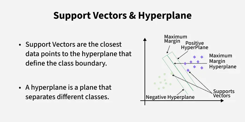
Support Vectors:
● Definition: Support vectors are the data points that lie closest to the decision boundary
(hyperplane). These points are the most challenging to classify correctly and are the key
points that define the position and orientation of the hyperplane.
Importance:
● The support vectors are critical because they are the points that “support” the optimal
hyperplane. In fact, the SVM model is entirely defined by these support vectors. The position
of all other data points is irrelevant as long as they are correctly classified by the hyperplane.

● If you remove a support vector from the dataset, the hyperplane could shift, potentially
changing the classification of some other points. However, removing a non-support vector
point will not affect the hyperplane.

2. Margin Maximization:
   ● Definition: The margin is the distance between the hyperplane and the nearest data points
   from any class (i.e., the support vectors). In a binary classification problem, there will be a
   margin on either side of the hyperplane.
   ● Objective of SVM: SVM aims to find the hyperplane that maximizes this margin, making the
   classifier as robust as possible.
   ● Why Maximize the Margin?:
   o Generalization: A larger margin implies that the model has more confidence in its
   classification decisions. It reduces the risk of overfitting because the model is less
   sensitive to slight variations in the data points.
   o Robustness: A wider margin means the model is better at generalizing to unseen
   data. If new data points are added, they are more likely to be classified correctly if the margin is large.
3. Mathematical Perspective
   𝐷𝑖𝑠𝑡𝑎𝑛𝑐𝑒 𝑏𝑒𝑡𝑤𝑒𝑒𝑛 𝑠𝑢𝑝𝑝𝑜𝑟𝑡 𝑣𝑒𝑐𝑡𝑜𝑟 𝑑𝑎𝑡𝑎𝑝𝑜𝑖𝑛𝑡𝑠 𝑡𝑜 ℎ𝑦𝑝𝑒𝑟 𝑝𝑙𝑎𝑛𝑒 𝑖𝑠 𝑔𝑖𝑣𝑒𝑛 𝑏𝑦
   𝑑 =𝑤1𝑥1+𝑤2𝑦1+𝑤𝑜| |𝑤12+𝑤2

2

𝑤1𝑥1+𝑤2𝑦1+𝑤𝑜| | ||𝑊|| =𝑤𝑜+𝑤𝑇𝑥||||||||𝑊||
𝑀𝑎𝑟𝑔𝑖𝑛
𝑤𝑜+𝑤𝑇𝑥||||||||𝑊||
𝑑𝑟 = ||𝑊|| 𝑚𝑖𝑛𝑖𝑢𝑚 𝑐𝑜𝑛𝑠𝑡𝑟𝑎𝑖𝑛 𝑡𝑜 𝑦 * 𝑤𝑜 + 𝑤
𝑇( 𝑥)≥1

𝑂𝑝𝑡𝑖𝑚𝑖𝑧𝑎𝑡𝑖𝑜𝑛:
𝑀𝑖𝑛𝑖𝑚𝑖𝑧𝑒 𝑡ℎ𝑒 = ||𝑊|| 𝑓𝑜𝑟 𝑚𝑎𝑡ℎ 𝑠𝑖𝑚𝑝𝑙𝑖𝑐𝑖𝑡𝑦 𝑖𝑛 𝑡𝑒𝑥𝑡 𝑏𝑜𝑜𝑘𝑠 𝑟𝑒𝑡𝑢𝑟𝑛 𝑎𝑠 =12 𝑤2
𝑀𝑖𝑛𝑖𝑚𝑖𝑧𝑒 𝑡ℎ𝑒 𝑡ℎ𝑒 12 𝑤2
𝑠𝑢𝑏𝑗𝑒𝑐𝑡 𝑡𝑜 𝑡ℎ𝑒 𝑐𝑜𝑛𝑠𝑡𝑟𝑎𝑖𝑛 𝑦 * 𝑤𝑜 + 𝑤
𝑇( 𝑥)𝐿(𝑥, 𝑦, λ) = 𝑓(𝑥, 𝑦) − λ * 𝑔(𝑥, 𝑦)𝐿 𝑤𝑜
( , 𝑤, λ) = ||𝑊|| − λ * [𝑦 * 𝑤𝑜 + 𝑤𝑇( 𝑥) − 1]𝐿 𝑏
𝑜( , 𝑤, λ) = ||𝑊|| − λ * [𝑦 * 𝑏𝑜 + 𝑤𝑇( 𝑥) − 1]𝐿 𝑏𝑜( , 𝑏, λ) = ||𝑊|| − λ * [𝑦 * 𝑏𝑜 + 𝑏𝑇( 𝑥) − 1]
𝐹𝑜𝑟 𝑚𝑎𝑛𝑦 𝑑𝑎𝑡𝑎𝑝𝑜𝑖𝑛𝑡𝑠
𝐿 𝑤𝑜( , 𝑤, λ) = ||𝑊|| −𝑖=1𝑛∑ λ𝑖

[𝑦𝑖𝑤𝑜 + 𝑤 * 𝑥𝑖( ) − 1]𝐿 𝑤𝑜( , 𝑤, λ) =12 𝑤2 −𝑖=1𝑛∑ λ𝑖[𝑦𝑖𝑤𝑜 + 𝑤 * 𝑥𝑖( ) − 1]

• 𝑤ℎ𝑒𝑟𝑒 λ𝑖 𝑖𝑠 𝑡ℎ𝑒 𝐿𝑎𝑔𝑟𝑎𝑛𝑔𝑒 𝑚𝑢𝑙𝑡𝑖𝑝𝑙𝑖𝑒𝑟𝑠 𝑎𝑠𝑠𝑜𝑐𝑖𝑎𝑡𝑒𝑑 𝑤𝑖𝑡ℎ 𝑒𝑎𝑐ℎ 𝑐𝑜𝑛𝑠𝑡𝑟𝑎𝑖𝑛𝑡
  𝐶𝑎𝑠𝑒 − 1:𝑑𝐿𝑑𝑤 = 0
  𝑑𝐿𝑑𝑤 = 𝑤 −𝑖=1𝑛∑ λ𝑖 𝑦𝑖𝑥𝑖 = 0
• 𝑤 =𝑖=1𝑛∑ λ𝑖𝑦𝑖𝑥𝑖
  𝑇ℎ𝑖𝑠 𝑠ℎ𝑜𝑤𝑠 𝑡ℎ𝑎𝑡 𝑡ℎ𝑒 𝑤𝑒𝑖𝑔ℎ𝑡 𝑣𝑒𝑐𝑡𝑜𝑟 𝑤 𝑖𝑠 𝑎 𝑙𝑖𝑛𝑒𝑎𝑟 𝑐𝑜𝑚𝑏𝑖𝑛𝑎𝑡𝑖𝑜𝑛 𝑜𝑓 𝑡ℎ𝑒 𝑡𝑟𝑎𝑖𝑛𝑖𝑛𝑔 𝑒𝑥𝑎𝑚𝑝𝑙𝑒𝑠,
  𝑤ℎ𝑒𝑟𝑒 𝑡ℎ𝑒 𝑐𝑜𝑒𝑓𝑓𝑖𝑐𝑖𝑒𝑛𝑡𝑠 𝑎𝑟𝑒 𝑔𝑖𝑣𝑒𝑛 𝑏𝑦 𝑡ℎ𝑒 𝐿𝑎𝑔𝑟𝑎𝑛𝑔𝑒 𝑚𝑢𝑙𝑡𝑖𝑝𝑙𝑖𝑒𝑟𝑠 λ𝑖.

𝐶𝑎𝑠𝑒 − 2: 𝑑𝐿𝑑𝑤𝑜= 0𝐿 𝑤𝑜( , 𝑤, λ) =12 𝑤2 −𝑖=1𝑛∑ λ𝑖[𝑦𝑖𝑤𝑜 + 𝑤 * 𝑥𝑖( ) −1]𝑑𝐿𝑑𝑤𝑜=−𝑖=1𝑛∑λ𝑖𝑦𝑖=0𝑖=1𝑛∑λ𝑖𝑦𝑖 = 0
𝑁𝑜𝑤 𝑠𝑢𝑏𝑠𝑡𝑖𝑢𝑡𝑒 𝑤 =𝑖=1𝑛 ∑λ𝑖𝑦𝑖𝑥𝑖
𝑜𝑛 𝐿𝑒𝑔𝑟𝑎𝑛𝑔𝑒𝑠 𝑒𝑞𝑢𝑎𝑡𝑖𝑜𝑛
𝐿 𝑤𝑜( , 𝑤, λ) =12 𝑤2 −𝑖=1𝑛∑ λ𝑖[𝑦𝑖𝑤𝑜 + 𝑤 * 𝑥𝑖( ) − 1] 𝑚𝑎𝑥𝑖𝑚𝑖𝑧𝑒

• 𝑖=1𝑛∑ λ𝑖 −12𝑗=1𝑛∑𝑗=1𝑛∑ λ𝑖λ𝑗𝑦𝑖 𝑦𝑗(𝑥𝑖,𝑥𝑗) 𝑠𝑢𝑏𝑗𝑒𝑐𝑡 𝑡𝑜
• 𝑖=1𝑛∑ λ𝑖𝑦𝑖 = 0𝑥𝑖 𝑥𝑗 𝑑𝑎𝑡𝑎 𝑝𝑜𝑖𝑛𝑡𝑠 𝑦𝑖𝑦𝑗 𝑐𝑙𝑎𝑠𝑠𝑒𝑠 𝑏𝑜𝑡ℎ 𝑎𝑟𝑒 𝑎𝑣𝑎𝑖𝑙𝑎𝑏𝑙𝑒 𝑖𝑛 𝑎 𝑑𝑎𝑡𝑎𝑏𝑦 𝑎𝑝𝑝𝑙𝑦𝑖𝑛𝑔 𝑎𝑙𝑙 𝑜𝑢𝑟 𝑑𝑎𝑡𝑎 𝑝𝑜𝑖𝑛𝑡𝑠 𝑤𝑒 𝑐𝑎𝑛 𝑔𝑒𝑡 λ𝑖 𝑓𝑜𝑟 𝑒𝑎𝑐ℎ 𝑑𝑎𝑡𝑎 𝑝𝑜𝑖𝑛𝑡 𝑤𝑒 𝑤𝑖𝑙𝑙 𝑔𝑒𝑡 λ.
• 𝑇ℎ𝑒 𝑔𝑜𝑎𝑙 𝑖𝑠 𝑛𝑜𝑤 𝑡𝑜 𝑓𝑖𝑛𝑑 𝑡ℎ𝑒 𝑜𝑝𝑡𝑖𝑚𝑎𝑙 λ.
• 𝑇ℎ𝑒 λ𝑖 𝑣𝑎𝑙𝑢𝑒𝑠 𝑑𝑒𝑡𝑒𝑟𝑚𝑖𝑛𝑒 𝑤ℎ𝑖𝑐ℎ 𝑑𝑎𝑡𝑎 𝑝𝑜𝑖𝑛𝑡𝑠 𝑎𝑟𝑒 𝑠𝑢𝑝𝑝𝑜𝑟𝑡 𝑣𝑒𝑐𝑡𝑜𝑟𝑠 𝑖. 𝑒 λ𝑖 0

𝑗=1 𝑛 ∑𝑗=1 𝑛 ∑λ𝑖 λ𝑗𝑦𝑖𝑦𝑗(𝑥𝑖 𝑥𝑗)𝑤12

• 𝑤22 = ||𝑤|| = (𝑊 * 𝑊)12 =12 𝑤 * 𝑤

𝐿(𝑥, 𝑦, λ) =12 𝑤 * 𝑤 − λ * 𝑦 * 𝑤𝑜 + 𝑤𝑇( 𝑥)
𝑆𝑡𝑒𝑝 − 1: 𝑀𝑎𝑘𝑒 𝑡ℎ𝑒 𝑐𝑙𝑎𝑠𝑠𝑒𝑠 𝑒𝑞𝑢𝑎𝑡𝑖𝑜𝑛 𝑦 𝑤𝑜 + 𝑤𝑇( * 𝑥) > 1
𝑦 = 1 𝑐𝑙𝑎𝑠𝑠 1 𝑒𝑞𝑢𝑎𝑡𝑖𝑜𝑛 𝑤𝑜 + 𝑤𝑇

• 𝑥 > 1
  𝑦 =− 1 𝑐𝑙𝑎𝑠𝑠 2
  𝑒𝑞𝑢𝑎𝑡𝑖𝑜𝑛 𝑤𝑜 + 𝑤𝑇
• 𝑥 < 1
  𝑆𝑡𝑒𝑝 − 2: 𝐼𝑛𝑐𝑟𝑒𝑎𝑠𝑒 𝑡ℎ𝑒 𝑚𝑎𝑟𝑔𝑖𝑛 𝑑𝑖𝑠𝑡𝑎𝑛𝑐𝑒 𝑜𝑓 𝑡ℎ𝑒 𝑑𝑎𝑡𝑎 𝑝𝑜𝑖𝑛𝑡 𝑡𝑜 𝑡ℎ𝑒 ℎ𝑦𝑝𝑒𝑟𝑝𝑙𝑎𝑛𝑒
  𝑑 =𝑤1𝑥1+𝑤2𝑦1+𝑤𝑜| |𝑤12+𝑤2
• 𝑤1𝑥1+𝑤2𝑦1+𝑤𝑜| | ||𝑊|| =𝑤𝑜+𝑤𝑇𝑥||||||||𝑊||
• 𝑆𝑡𝑒𝑝 − 3: 𝐷𝑒𝑐𝑟𝑒𝑎𝑠𝑒 𝑡ℎ𝑒 ||𝑤||
• 𝑆𝑡𝑒𝑝 − 4: 𝐷𝑒𝑐𝑟𝑒𝑎𝑠𝑒 𝑡ℎ𝑒 ||𝑤|| 𝑏𝑎𝑠𝑒𝑑 𝑜𝑛 𝑐𝑜𝑛𝑠𝑡𝑟𝑎𝑖𝑛 𝑦 𝑤𝑜 + 𝑤𝑇
• ( * 𝑥) > 1 𝑎𝑝𝑝𝑙𝑦 𝑙𝑒𝑔𝑟𝑎𝑛𝑔𝑒𝑠
• 𝑥𝑖𝑦𝑖

(2, 2) 1
(4, 4) 1
(4, 0) -1
(0, 0) 1
𝑥𝑖λ
(2, 2) 0.25
(4, 4) 0
(4, 0) 0.25
(0, 0) 0
𝑠𝑜 𝑠𝑢𝑝𝑝𝑜𝑟𝑡 𝑣𝑒𝑐𝑡𝑜𝑟𝑠 𝑎𝑟𝑒 (2, 2)𝑎𝑛𝑑 (4, 0)

𝑤 =
𝑖=1𝑛∑ λ𝑖𝑦𝑖𝑥
𝑖 = 0. 25 * 1 * (2, 2) + 0. 25 * (− 1) * (4, 0) = (0. 5, 0. 5) − (1, 0) = (0. 5 − 1, 0. 5 − 0(−0.5𝑤𝑜+ 𝑤𝑇𝑥 = 1𝑤𝑜 + 𝑤1

• 𝑥1 + 𝑤2
• 𝑥2 = 1
  𝑤𝑜 − 0. 5 * 2 + 0. 5 * 2 = 1
  𝑤𝑜 − 1 + 1 = 1
  𝑤𝑜 = 1− 0. 5 * 𝑥1 + 0. 5 * 𝑥2 + 1

What Is a Support Vector Machine?
Support Vector Machine is designed to find the optimal hyperplane that separates data points of different classes with the maximum margin. It’s especially effective in high-dimensional spaces and for problems where the decision boundary is not linear.

🔍 Key Concepts

• Hyperplane: A decision boundary that separates different classes. In 2D, it’s a line; in 3D, it’s a plane.
• Support Vectors: The data points closest to the hyperplane. These are critical in defining the margin.
• Margin: The distance between the hyperplane and the support vectors. SVM aims to maximize this.
• Kernel Trick: A method to transform data into higher dimensions to make it linearly separable. Common kernels include linear, polynomial, and radial basis function (RBF).
• Hard Margin vs. Soft Margin:
• Hard Margin: Assumes perfect separation with no misclassification.
• Soft Margin: Allows some misclassification to handle noisy data better.
• Regularization (C): Controls the trade-off between maximizing the margin and minimizing classification error.

⚙️ How It Works

1. SVM identifies the hyperplane that best separates the classes.
2. It uses support vectors to define the margin.
3. If data isn’t linearly separable, it applies the kernel trick to map it into a higher-dimensional space.
4. Solves an optimization problem to find the best hyperplane.

Support Vector Machine (SVM) is a supervised machine learning algorithm used for classification and regression tasks. It tries to find the best boundary known as hyperplane that separates different classes in the data. It is useful when you want to do binary classification like spam vs. not spam or cat vs. dog.

The main goal of SVM is to maximize the margin between the two classes. The larger the margin the better the model performs on new and unseen data.

Key Concepts of Support Vector Machine

• Hyperplane: A decision boundary separating different classes in feature space and is represented by the equation wx + b = 0 in linear classification.
• Support Vectors: The closest data points to the hyperplane, crucial for determining the hyperplane and margin in SVM.
• Margin: The distance between the hyperplane and the support vectors. SVM aims to maximize this margin for better classification performance.
• Kernel: A function that maps data to a higher-dimensional space enabling SVM to handle non-linearly separable data.
• Hard Margin: A maximum-margin hyperplane that perfectly separates the data without misclassifications.
• Soft Margin: Allows some misclassifications by introducing slack variables, balancing margin maximization and misclassification penalties when data is not perfectly separable.
• C: A regularization term balancing margin maximization and misclassification penalties. A higher C value forces stricter penalty for misclassifications.
• Hinge Loss: A loss function penalizing misclassified points or margin violations and is combined with regularization in SVM.
• Dual Problem: Involves solving for Lagrange multipliers associated with support vectors, facilitating the kernel trick and efficient computation.

How does Support Vector Machine Algorithm Work?

The key idea behind the SVM algorithm is to find the hyperplane that best separates two classes by maximizing the margin between them. This margin is the distance from the hyperplane to the nearest data points (support vectors) on each side.

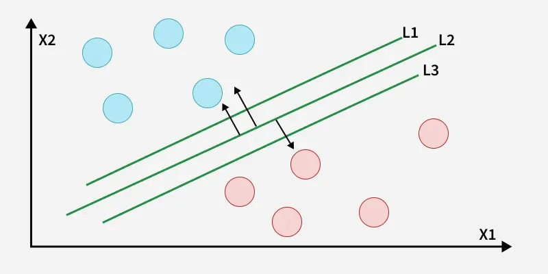
The best hyperplane also known as the “hard margin” is the one that maximizes the distance between the hyperplane and the nearest data points from both classes. This ensures a clear separation between the classes. So from the above figure, we choose L2 as hard margin. Let’s consider a scenario like shown below:

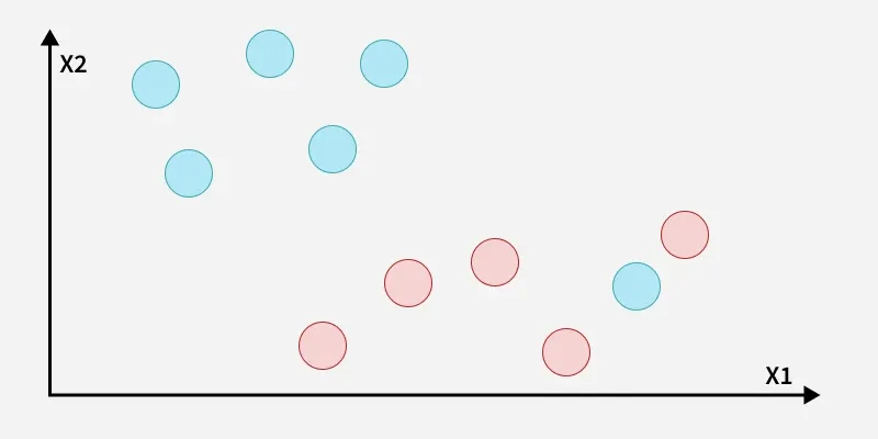
Here, we have one blue ball in the boundary of the red ball.

How does SVM classify the data?

The blue ball in the boundary of red ones is an outlier of blue balls. The SVM algorithm has the characteristics to ignore the outlier and finds the best hyperplane that maximizes the margin. SVM is robust to outliers.

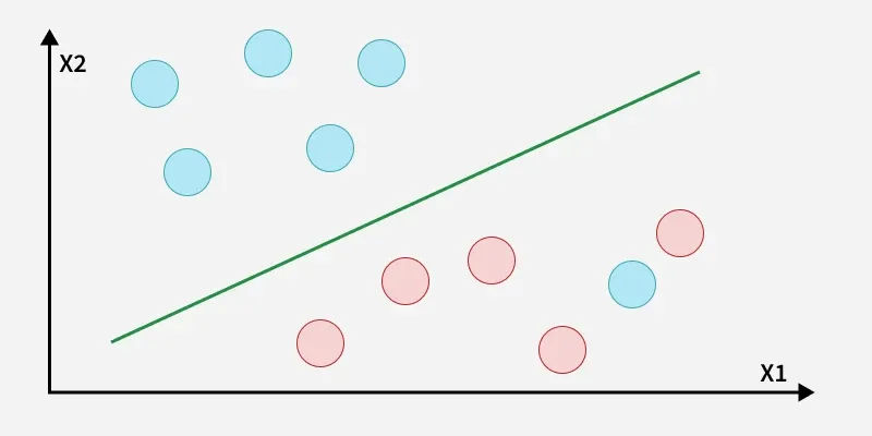
A soft margin allows for some misclassifications or violations of the margin to improve generalization. The SVM optimizes the following equation to balance margin maximization and penalty minimization:

Objective Function=(1margin)+λ∑penalty Objective Function=(margin1​)+λ∑penalty 

The penalty used for violations is often hinge loss which has the following behavior:

• If a data point is correctly classified and within the margin there is no penalty (loss = 0).
• If a point is incorrectly classified or violates the margin the hinge loss increases proportionally to the distance of the violation.

Till now we were talking about linearly separable data that seprates group of blue balls and red balls by a straight line/linear line.

What if data is not linearly separable?

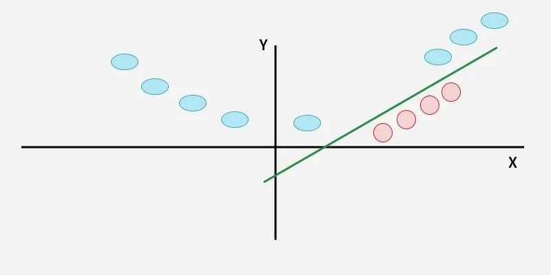
When data is not linearly separable i.e it can’t be divided by a straight line, SVM uses a technique called kernels to map the data into a higher-dimensional space where it becomes separable. This transformation helps SVM find a decision boundary even for non-linear data.

A kernel is a function that maps data points into a higher-dimensional space without explicitly computing the coordinates in that space. This allows SVM to work efficiently with non-linear data by implicitly performing the mapping. For example consider data points that are not linearly separable. By applying a kernel function SVM transforms the data points into a higher-dimensional space where they become linearly separable.

• Linear Kernel: For linear separability.
• Polynomial Kernel: Maps data into a polynomial space.
• Radial Basis Function (RBF) Kernel: Transforms data into a space based on distances between data points.

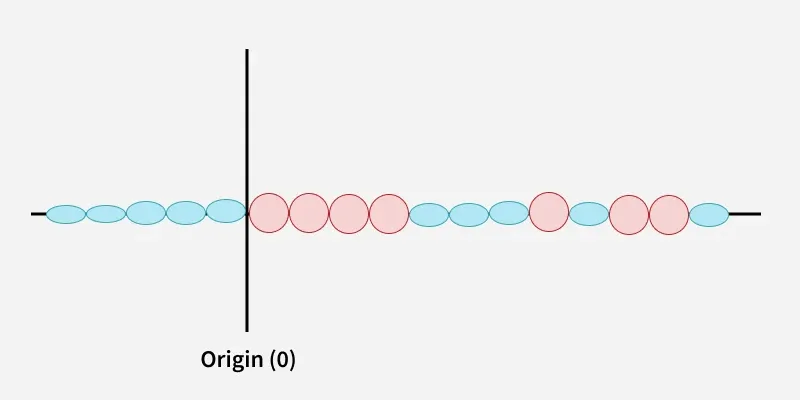
In this case the new variable y is created as a function of distance from the origin.

Mathematical Computation of SVM

Consider a binary classification problem with two classes, labeled as +1 and -1. We have a training dataset consisting of input feature vectors X and their corresponding class labels Y. The equation for the linear hyperplane can be written as:

wTx+b=0wTx+b=0

Where:

• ww is the normal vector to the hyperplane (the direction perpendicular to it).
• bb is the offset or bias term representing the distance of the hyperplane from the origin along the normal vector ww.

Distance from a Data Point to the Hyperplane

The distance between a data point xixi​and the decision boundary can be calculated as:

di=wTxi+b∣∣w∣∣di​=∣∣w∣∣wTxi​+b​

where ||w|| represents the Euclidean norm of the weight vector w.

Linear SVM Classifier

Distance from a Data Point to the Hyperplane:

y^={1: wTx+b≥00:  wTx+b <0y^​={10​: wTx+b≥0:  wTx+b <0​

Where y^y^​ is the predicted label of a data point.

Optimization Problem for SVM

For a linearly separable dataset the goal is to find the hyperplane that maximizes the margin between the two classes while ensuring that all data points are correctly classified. This leads to the following optimization problem:

minimizew,b12∥w∥2w,bminimize​21​∥w∥2

Subject to the constraint:

yi(wTxi+b)≥1fori=1,2,3,⋯,myi​(wTxi​+b)≥1fori=1,2,3,⋯,m

Where:

• yiyi​​ is the class label (+1 or -1) for each training instance.
• xixi​​ is the feature vector for the ii-th training instance.
• mm is the total number of training instances.

The condition yi(wTxi+b)≥1yi​(wTxi​+b)≥1 ensures that each data point is correctly classified and lies outside the margin.

Soft Margin in Linear SVM Classifier

In the presence of outliers or non-separable data the SVM allows some misclassification by introducing slack variables ζiζi​​. The optimization problem is modified as:

minimize w,b12∥w∥2+C∑i=1mζiw,bminimize ​21​∥w∥2+C∑i=1m​ζi​

Subject to the constraints:

yi(wTxi+b)≥1−ζiandζi≥0for i=1,2,…,myi​(wTxi​+b)≥1−ζi​andζi​≥0for i=1,2,…,m

Where:

• CC is a regularization parameter that controls the trade-off between margin maximization and penalty for misclassifications.
• ζiζi​​ are slack variables that represent the degree of violation of the margin by each data point.

Dual Problem for SVM

The dual problem involves maximizing the Lagrange multipliers associated with the support vectors. This transformation allows solving the SVM optimization using kernel functions for non-linear classification.

The dual objective function is given by:

maximize α12∑i=1m∑j=1mαiαjtitjK(xi,xj)−∑i=1mαiαmaximize ​21​∑i=1m​∑j=1m​αi​αj​ti​tj​K(xi​,xj​)−∑i=1m​αi​

Where:

• αiαi​​ are the Lagrange multipliers associated with the ithith training sample.
• titi​​ is the class label for the ithith-th training sample.
• K(xi,xj)K(xi​,xj​) is the kernel function that computes the similarity between data points xixi​​ and xjxj​​. The kernel allows SVM to handle non-linear classification problems by mapping data into a higher-dimensional space.

The dual formulation optimizes the Lagrange multipliers αiαi​​ and the support vectors are those training samples where αi>0αi​>0.

SVM Decision Boundary

Once the dual problem is solved, the decision boundary is given by:

w=∑i=1mαitiK(xi,x)+bw=∑i=1m​αi​ti​K(xi​,x)+b

Where ww is the weight vector, xx is the test data point and bb is the bias term. Finally the bias term bb is determined by the support vectors, which satisfy:

ti(wTxi−b)=1⇒b=wTxi−titi​(wTxi​−b)=1⇒b=wTxi​−ti​

Where xixi​​ is any support vector.

This completes the mathematical framework of the Support Vector Machine algorithm which allows for both linear and non-linear classification using the dual problem and kernel trick.

Types of Support Vector Machine

Based on the nature of the decision boundary, Support Vector Machines (SVM) can be divided into two main parts:

• Linear SVM: Linear SVMs use a linear decision boundary to separate the data points of different classes. When the data can be precisely linearly separated, linear SVMs are very suitable. This means that a single straight line (in 2D) or a hyperplane (in higher dimensions) can entirely divide the data points into their respective classes. A hyperplane that maximizes the margin between the classes is the decision boundary.
• Non-Linear SVM: Non-Linear SVM can be used to classify data when it cannot be separated into two classes by a straight line (in the case of 2D). By using kernel functions, nonlinear SVMs can handle nonlinearly separable data. The original input data is transformed by these kernel functions into a higher-dimensional feature space where the data points can be linearly separated. A linear SVM is used to locate a nonlinear decision boundary in this modified space. 

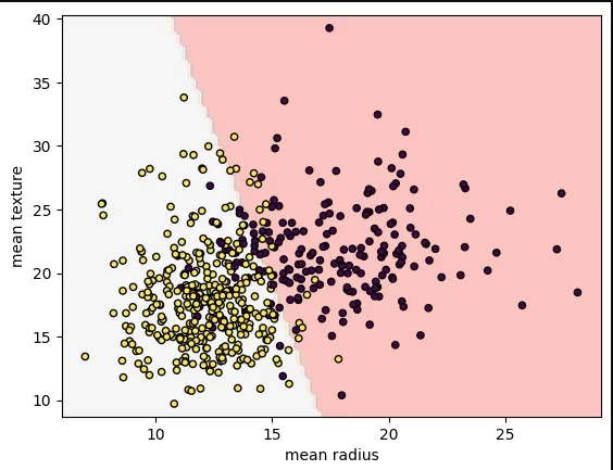
Implementing SVM Algorithm Using Scikit-Learn

We will predict whether cancer is Benign or Malignant using historical data about patients diagnosed with cancer. This data includes independent attributes such as tumor size, texture, and others. To perform this classification, we will use an SVM (Support Vector Machine) classifier to differentiate between benign and malignant cases effectively.

• load_breast_cancer(): Loads the breast cancer dataset (features and target labels).
• SVC(kernel=”linear”, C=1): Creates a Support Vector Classifier with a linear kernel and regularization parameter C=1.
• svm.fit(X, y): Trains the SVM model on the feature matrix X and target labels y.
• DecisionBoundaryDisplay.from_estimator(): Visualizes the decision boundary of the trained model with a specified color map.
• plt.scatter(): Creates a scatter plot of the data points, colored by their labels.
• plt.show(): Displays the plot to the screen.

from sklearn.datasets import load_breast_cancer import matplotlib.pyplot as plt from sklearn.inspection import DecisionBoundaryDisplay from sklearn.svm import SVC cancer = load_breast_cancer() X = cancer.data[:, :2] y = cancer.target svm = SVC(kernel="linear", C=1) svm.fit(X, y) DecisionBoundaryDisplay.from_estimator( svm, X, response_method="predict", alpha=0.8, cmap="Pastel1", xlabel=cancer.feature_names[0], ylabel=cancer.feature_names[1], ) plt.scatter(X[:, 0], X[:, 1], c=y, s=20, edgecolors="k") plt.show()

Output:

Advantages of Support Vector Machine (SVM)

1. High-Dimensional Performance: SVM excels in high-dimensional spaces, making it suitable for image classification and gene expression analysis.
2. Nonlinear Capability: Utilizing kernel functions like RBF and polynomial SVM effectively handles nonlinear relationships.
3. Outlier Resilience: The soft margin feature allows SVM to ignore outliers, enhancing robustness in spam detection and anomaly detection.
4. Binary and Multiclass Support: SVM is effective for both binary classification and multiclass classification suitable for applications in text classification.
5. Memory Efficiency: It focuses on support vectors making it memory efficient compared to other algorithms.

Disadvantages of Support Vector Machine (SVM)

1. Slow Training: SVM can be slow for large datasets, affecting performance in SVM in data mining tasks.
2. Parameter Tuning Difficulty: Selecting the right kernel and adjusting parameters like C requires careful tuning, impacting SVM algorithms.
3. Noise Sensitivity: SVM struggles with noisy datasets and overlapping classes, limiting effectiveness in real-world scenarios.
4. Limited Interpretability: The complexity of the hyperplane in higher dimensions makes SVM less interpretable than other models.
5. Feature Scaling Sensitivity: Proper feature scaling is essential, otherwise SVM models may perform poorly.