BERT Model Embedding Vector Under stabbing
A “BERT Model Embedding Vector” is a numerical representation of words or sentences generated by Google’s BERT (Bidirectional Encoder Representations from Transformers) model, which captures their contextual meaning. These high-dimensional vectors encode information about a word or sentence, allowing computers to understand and process human language for various NLP tasks. Each token (word or subword) in a sentence gets a unique vector, with the final embedding for a sentence often derived by combining token-level embeddings.
BERT Model for Text Embeddings
This notebook demonstrates how to use the BERT (Bidirectional Encoder Representations from Transformers) model for text embeddings using the TensorFlow framework. BERT is a pre-trained deep learning model that has achieved state-of-the-art performance on various natural language processing tasks.
In this notebook, we will walk through the process of loading the BERT preprocessor and encoder, preprocessing text inputs, passing the inputs through the BERT model, and extracting text embeddings. Text embeddings capture the semantic meaning of words or sentences in a dense vector representation, enabling various downstream tasks such as sentiment analysis, text classification, and information retrieval.
1| Install the necessary libraries
This step installs the required libraries: TensorFlow, TensorFlow Hub, and TensorFlow Text.
These libraries are necessary for working with the BERT model and performing text embedding tasks.
!pip install tensorflow tensorflow_hub tensorflow_text"
/bin/bash: -c: line 0: unexpected EOF while looking for matching `"'
/bin/bash: -c: line 1: syntax error: unexpected end of file
import numpy as np # linear algebra
import pandas as pd # data processing, CSV file I/O (e.g. pd.read_csv)
2: Import the required libraries
Here, we import the TensorFlow, TensorFlow Hub, and TensorFlow Text libraries to access the BERT model and related functionalities.
import tensorflow as tf
import tensorflow_hub as hub
import tensorflow_text as text
/opt/conda/lib/python3.10/site-packages/tensorflow_io/python/ops/__init__.py:98: UserWarning: unable to load libtensorflow_io_plugins.so: unable to open file: libtensorflow_io_plugins.so, from paths: ['/opt/conda/lib/python3.10/site-packages/tensorflow_io/python/ops/libtensorflow_io_plugins.so']
caused by: ['/opt/conda/lib/python3.10/site-packages/tensorflow_io/python/ops/libtensorflow_io_plugins.so: undefined symbol: _ZN3tsl6StatusC1EN10tensorflow5error4CodeESt17basic_string_viewIcSt11char_traitsIcEENS_14SourceLocationE']
  warnings.warn(f"unable to load libtensorflow_io_plugins.so: {e}")
/opt/conda/lib/python3.10/site-packages/tensorflow_io/python/ops/__init__.py:104: UserWarning: file system plugins are not loaded: unable to open file: libtensorflow_io.so, from paths: ['/opt/conda/lib/python3.10/site-packages/tensorflow_io/python/ops/libtensorflow_io.so']
caused by: ['/opt/conda/lib/python3.10/site-packages/tensorflow_io/python/ops/libtensorflow_io.so: undefined symbol: _ZTVN10tensorflow13GcsFileSystemE']
  warnings.warn(f"file system plugins are not loaded: {e}")
3| Define the input layer
This line defines an input layer for the text data. It specifies that the input shape is an empty tensor with a string data type.
text_input = tf.keras.layers.Input(shape=(), dtype=tf.string)
4| Load the BERT preprocessor
We load the BERT preprocessor from TensorFlow Hub. The preprocessor handles the text preprocessing tasks required by the BERT model, such as tokenization and input formatting.
preprocessor = hub.KerasLayer(
    "https://tfhub.dev/tensorflow/bert_en_uncased_preprocess/3")
5| Preprocess the input using the BERT preprocessor
This line preprocesses the input text using the BERT preprocessor. It applies tokenization, converts the text into BERT-compatible input tensors, and returns the preprocessed input tensors.
encoder_inputs = preprocessor(text_input)
6| Load the BERT encoder
We load the BERT encoder from TensorFlow Hub. The encoder is the main BERT model responsible for generating text embeddings.
encoder = hub.KerasLayer(
    "https://tfhub.dev/tensorflow/bert_en_uncased_L-12_H-768_A-12/4",
    trainable=True)
7| Pass the preprocessed inputs through the BERT encoder
This line passes the preprocessed input tensors through the BERT encoder to obtain the model’s outputs. The outputs include the pooled_output and sequence_output.
outputs = encoder(encoder_inputs)
8| Extract the pooled_output and sequence_output
Here, we extract the pooled_output and sequence_output from the outputs of the BERT encoder.
The pooled_output represents the entire input sequence, while the sequence_output represents each token in the context of the input sequence.
pooled_output = outputs["pooled_output"]      # [batch_size, 768]
sequence_output = outputs["sequence_output"]  # [batch_size, seq_length, 768]
9| Define the model and compile it (optional)
This step defines the model using the Keras functional API. We specify the input layer as text_input and the output layer as pooled_output. Optionally, we can compile the model by specifying an optimizer and loss function.
embedding_model = tf.keras.Model(text_input, pooled_output)
embedding_model.compile(optimizer='adam', loss='mse')
10| Use the BERT model for text embeddings
we use the embedding_model to obtain text embeddings for a list of example sentences. We pass the sentences to the embedding_model and store the resulting embeddings in the embeddings variable.
sentences = tf.constant(["Example sentence 1", "Example sentence 2"])
embeddings = embedding_model(sentences)
11| Print the embeddings
Finally, we print the obtained text embeddings to inspect the results.
The embeddings variable contains the text embeddings for the example sentences, which can be further processed or used for downstream tasks.
print(embeddings)
tf.Tensor(
[[-0.88612574 -0.2960122   0.14618956 ... -0.37177786 -0.5755337
   0.89689547]
 [-0.90233845 -0.36567798 -0.14331412 ... -0.5138187  -0.62246144
   0.9048834 ]], shape=(2, 768), dtype=float32)
What it is:
- Numerical Representation:A BERT embedding vector is a dense vector of numbers that represents the semantic meaning of a word or sentence.
Bidirectional encoder representations from transformers (BERT) is a language model introduced in October 2018 by researchers at Google.[1][2] It learns to represent text as a sequence of vectors using self-supervised learning. It uses the encoder-only transformer architecture. BERT dramatically improved the state of the art for large language models. As of 2020, BERT is a ubiquitous baseline in natural language processing (NLP) experiments.[3]
BERT is trained by masked token prediction and next sentence prediction. With this training, BERT learns contextual, latent representations of tokens in their context, similar to ELMo and GPT-2.[4] It found applications for many natural language processing tasks, such as coreference resolution and polysemy resolution.[5] It improved on ELMo and spawned the study of “BERTology”, which attempts to interpret what is learned by BERT.[3]
BERT was originally implemented in the English language at two model sizes, BERTBASE (110 million parameters) and BERTLARGE (340 million parameters). Both were trained on the Toronto BookCorpus[6] (800M words) and English Wikipedia (2,500M words).[1]: 5 The weights were released on GitHub.[7] On March 11, 2020, 24 smaller models were released, the smallest being BERTTINY with just 4 million parameters.[7]
Architecture

BERT is an “encoder-only” transformer architecture. At a high level, BERT consists of 4 modules:
- Tokenizer: This module converts a piece of English text into a sequence of integers (“tokens”).
- Embedding: This module converts the sequence of tokens into an array of real-valued vectors representing the tokens. It represents the conversion of discrete token types into a lower-dimensional Euclidean space.
- Encoder: a stack of Transformer blocks with self-attention, but without causal masking.
- Task head: This module converts the final representation vectors into one-hot encoded tokens again by producing a predicted probability distribution over the token types. It can be viewed as a simple decoder, decoding the latent representation into token types, or as an “un-embedding layer”.
The task head is necessary for pre-training, but it is often unnecessary for so-called “downstream tasks,” such as question answering or sentiment classification. Instead, one removes the task head and replaces it with a newly initialized module suited for the task, and finetune the new module. The latent vector representation of the model is directly fed into this new module, allowing for sample-efficient transfer learning.[1][8]

Embedding
This section describes the embedding used by BERTBASE. The other one, BERTLARGE, is similar, just larger.
The tokenizer of BERT is WordPiece, which is a sub-word strategy like byte-pair encoding. Its vocabulary size is 30,000, and any token not appearing in its vocabulary is replaced by [UNK] (“unknown”).

The first layer is the embedding layer, which contains three components: token type embeddings, position embeddings, and segment type embeddings.
- Token type: The token type is a standard embedding layer, translating a one-hot vector into a dense vector based on its token type.
- Position: The position embeddings are based on a token’s position in the sequence. BERT uses absolute position embeddings, where each position in a sequence is mapped to a real-valued vector. Each dimension of the vector consists of a sinusoidal function that takes the position in the sequence as input.
- Segment type: Using a vocabulary of just 0 or 1, this embedding layer produces a dense vector based on whether the token belongs to the first or second text segment in that input. In other words, type-1 tokens are all tokens that appear after the
[SEP]special token. All prior tokens are type-0.
The three embedding vectors are added together representing the initial token representation as a function of these three pieces of information. After embedding, the vector representation is normalized using a LayerNorm operation, outputting a 768-dimensional vector for each input token. After this, the representation vectors are passed forward through 12 Transformer encoder blocks, and are decoded back to 30,000-dimensional vocabulary space using a basic affine transformation layer.
Architectural family
The encoder stack of BERT has 2 free parameters: L


For BERT:
- the feed-forward size and filter size are synonymous. Both of them denote the number of dimensions in the middle layer of the feed-forward network.
- the hidden size and embedding size are synonymous. Both of them denote the number of real numbers used to represent a token.
The notation for encoder stack is written as L/H. For example, BERTBASE is written as 12L/768H, BERTLARGE as 24L/1024H, and BERTTINY as 2L/128H.
Training
Pre-training
BERT was pre-trained simultaneously on two tasks:[10]
- Masked language modeling (MLM): In this task, BERT ingests a sequence of words, where one word may be randomly changed (“masked”), and BERT tries to predict the original words that had been changed. For example, in the sentence “The cat sat on the
[MASK],” BERT would need to predict “mat.” This helps BERT learn bidirectional context, meaning it understands the relationships between words not just from left to right or right to left but from both directions at the same time. - Next sentence prediction (NSP): In this task, BERT is trained to predict whether one sentence logically follows another. For example, given two sentences, “The cat sat on the mat” and “It was a sunny day”, BERT has to decide if the second sentence is a valid continuation of the first one. This helps BERT understand relationships between sentences, which is important for tasks like question answering or document classification.
Masked language modeling

In masked language modeling, 15% of tokens would be randomly selected for masked-prediction task, and the training objective was to predict the masked token given its context. In more detail, the selected token is:
- replaced with a
[MASK]token with probability 80%, - replaced with a random word token with probability 10%,
- not replaced with probability 10%.
The reason not all selected tokens are masked is to avoid the dataset shift problem. The dataset shift problem arises when the distribution of inputs seen during training differs significantly from the distribution encountered during inference. A trained BERT model might be applied to word representation (like Word2Vec), where it would be run over sentences not containing any [MASK] tokens. It is later found that more diverse training objectives are generally better.[11]
As an illustrative example, consider the sentence “my dog is cute”. It would first be divided into tokens like “my1 dog2 is3 cute4“. Then a random token in the sentence would be picked. Let it be the 4th one “cute4“. Next, there would be three possibilities:
- with probability 80%, the chosen token is masked, resulting in “my1 dog2 is3
[MASK]4“; - with probability 10%, the chosen token is replaced by a uniformly sampled random token, such as “happy”, resulting in “my1 dog2 is3 happy4“;
- with probability 10%, nothing is done, resulting in “my1 dog2 is3 cute4“.
After processing the input text, the model’s 4th output vector is passed to its decoder layer, which outputs a probability distribution over its 30,000-dimensional vocabulary space.
Next sentence prediction

Given two sentences, the model predicts if they appear sequentially in the training corpus, outputting either [IsNext] or [NotNext]. During training, the algorithm sometimes samples two sentences from a single continuous span in the training corpus, while at other times, it samples two sentences from two discontinuous spans.
The first sentence starts with a special token, [CLS] (for “classify”). The two sentences are separated by another special token, [SEP] (for “separate”). After processing the two sentences, the final vector for the [CLS] token is passed to a linear layer for binary classification into [IsNext] and [NotNext].
For example:
- Given “
[CLS]my dog is cute[SEP]he likes playing[SEP]“, the model should predict[IsNext]. - Given “
[CLS]my dog is cute[SEP]how do magnets work[SEP]“, the model should predict[NotNext].
Fine-tuning
Fine-tuned tasks for BERT[12]
- Sentiment classification
- Sentence classification
- Answering multiple-choice questions
- Part-of-speech tagging
BERT is meant as a general pretrained model for various applications in natural language processing. That is, after pre-training, BERT can be fine-tuned with fewer resources on smaller datasets to optimize its performance on specific tasks such as natural language inference and text classification, and sequence-to-sequence-based language generation tasks such as question answering and conversational response generation.[12]
The original BERT paper published results demonstrating that a small amount of finetuning (for BERTLARGE, 1 hour on 1 Cloud TPU) allowed it to achieved state-of-the-art performance on a number of natural language understanding tasks:[1]
- GLUE (General Language Understanding Evaluation) task set (consisting of 9 tasks);
- SQuAD (Stanford Question Answering Dataset[13]) v1.1 and v2.0;
- SWAG (Situations With Adversarial Generations[14]).
In the original paper, all parameters of BERT are fine-tuned, and recommended that, for downstream applications that are text classifications, the output token at the [CLS] input token is fed into a linear-softmax layer to produce the label outputs.[1]
The original code base defined the final linear layer as a “pooler layer”, in analogy with global pooling in computer vision, even though it simply discards all output tokens except the one corresponding to [CLS] .[15]
Cost
BERT was trained on the BookCorpus (800M words) and a filtered version of English Wikipedia (2,500M words) without lists, tables, and headers.
Training BERTBASE on 4 cloud TPU (16 TPU chips total) took 4 days, at an estimated cost of 500 USD.[7] Training BERTLARGE on 16 cloud TPU (64 TPU chips total) took 4 days.[1]
Interpretation
Language models like ELMo, GPT-2, and BERT, spawned the study of “BERTology”, which attempts to interpret what is learned by these models. Their performance on these natural language understanding tasks are not yet well understood.[3][16][17] Several research publications in 2018 and 2019 focused on investigating the relationship behind BERT’s output as a result of carefully chosen input sequences,[18][19] analysis of internal vector representations through probing classifiers,[20][21] and the relationships represented by attention weights.[16][17]
The high performance of the BERT model could also be attributed to the fact that it is bidirectionally trained.[22] This means that BERT, based on the Transformer model architecture, applies its self-attention mechanism to learn information from a text from the left and right side during training, and consequently gains a deep understanding of the context. For example, the word fine can have two different meanings depending on the context (I feel fine today, She has fine blond hair). BERT considers the words surrounding the target word fine from the left and right side.
However it comes at a cost: due to encoder-only architecture lacking a decoder, BERT can’t be prompted and can’t generate text, while bidirectional models in general do not work effectively without the right side, thus being difficult to prompt. As an illustrative example, if one wishes to use BERT to continue a sentence fragment “Today, I went to”, then naively one would mask out all the tokens as “Today, I went to [MASK] [MASK] [MASK] … [MASK] .” where the number of [MASK] is the length of the sentence one wishes to extend to. However, this constitutes a dataset shift, as during training, BERT has never seen sentences with that many tokens masked out. Consequently, its performance degrades. More sophisticated techniques allow text generation, but at a high computational cost.[23]
History
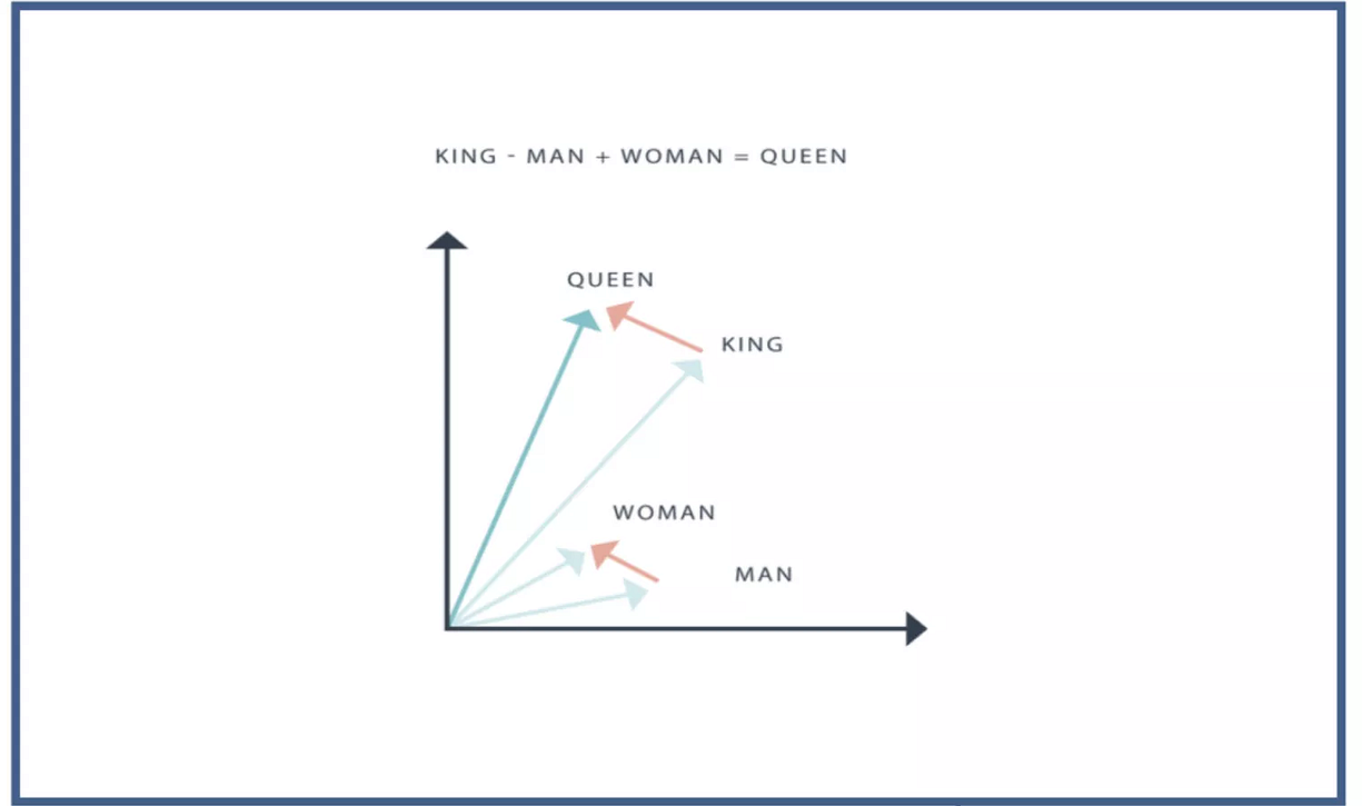
BERT was originally published by Google researchers Jacob Devlin, Ming-Wei Chang, Kenton Lee, and Kristina Toutanova. The design has its origins from pre-training contextual representations, including semi-supervised sequence learning,[24] generative pre-training, ELMo,[25] and ULMFit.[26] Unlike previous models, BERT is a deeply bidirectional, unsupervised language representation, pre-trained using only a plain text corpus. Context-free models such as word2vec or GloVe generate a single word embedding representation for each word in the vocabulary, whereas BERT takes into account the context for each occurrence of a given word. For instance, whereas the vector for “running” will have the same word2vec vector representation for both of its occurrences in the sentences “He is running a company” and “He is running a marathon”, BERT will provide a contextualized embedding that will be different according to the sentence.[4]
On October 25, 2019, Google announced that they had started applying BERT models to English-language search queries on Google Search within the US.[27] On December 9, 2019, it was reported that BERT had been adopted by Google Search for over 70 languages.[28][29] In October 2020, almost every single English-based query was processed by a BERT model.[30]
Variants
The BERT models were influential and inspired many variants.
RoBERTa (2019)[31] was an engineering improvement. It preserves BERT’s architecture (slightly larger, at 355M parameters), but improves its training, changing key hyperparameters, removing the next-sentence prediction task, and using much larger mini-batch sizes.
XLM-RoBERTa (2019)[32] was a multilingual RoBERTa model. It was one of the first works on multilingual language modeling at scale.
DistilBERT (2019) distills BERTBASE to a model with just 60% of its parameters (66M), while preserving 95% of its benchmark scores.[33][34] Similarly, TinyBERT (2019)[35] is a distilled model with just 28% of its parameters.
ALBERT (2019)[36] used shared-parameter across layers, and experimented with independently varying the hidden size and the word-embedding layer’s output size as two hyperparameters. They also replaced the next sentence prediction task with the sentence-order prediction (SOP) task, where the model must distinguish the correct order of two consecutive text segments from their reversed order.
ELECTRA (2020)[37] applied the idea of generative adversarial networks to the MLM task. Instead of masking out tokens, a small language model generates random plausible substitutions, and a larger network identify these replaced tokens. The small model aims to fool the large model.
DeBERTa (2020)[38] is a significant architectural variant, with disentangled attention. Its key idea is to treat the positional and token encodings separately throughout the attention mechanism. Instead of combining the positional encoding (xposition


| Attention type | Query type | Key type | Example |
|---|---|---|---|
| Content-to-content | Token | Token | “European”; “Union”, “continent” |
| Content-to-position | Token | Position | [adjective]; +1, +2, +3 |
| Position-to-content | Position | Token | −1; “not”, “very” |
The three attention matrices are added together element-wise, then passed through a softmax layer and multiplied by a projection matrix.
Absolute position encoding is included in the final self-attention layer as additional input.
- Contextual:Unlike older methods, BERT’s embeddings are contextual, meaning the vector for a word changes depending on the surrounding words in the sentence. For example, the word “bank” will have different embeddings in “river bank” and “bank robber”.
BERT Input
BERT can take as input either one or two sentences, and uses the special token [SEP] to differentiate them. The [CLS] token always appears at the start of the text, and is specific to classification tasks.
Both tokens are always required, even if we only have one sentence, and even if we are not using BERT for classification. That’s how BERT was pre-trained, and so that’s what BERT expects to see.
2 Sentence Input:
[CLS] The man went to the store. [SEP] He bought a gallon of milk.
1 Sentence Input:
[CLS] The man went to the store. [SEP]
Tokenization and Word Embedding
Next let’s take a look at how we convert the words into numerical representations.
We first take the sentence and tokenize it.
text = "Here is the sentence I want embeddings for."
marked_text = "[CLS] " + text + " [SEP]"# Tokenize our sentence with the BERT tokenizer.
tokenized_text = tokenizer.tokenize(marked_text)# Print out the tokens.
print (tokenized_text)['[CLS]', 'here', 'is', 'the', 'sentence', 'i', 'want', 'em', '##bed', '##ding', '##s', 'for', '.', '[SEP]']
Notice how the word “embeddings” is represented:
['em', '##bed', '##ding', '##s']
The original word has been split into smaller subwords and characters. This is because Bert Vocabulary is fixed with a size of ~30K tokens. Words that are not part of vocabulary are represented as subwords and characters.
Tokenizer takes the input sentence and will decide to keep every word as a whole word, split it into sub words(with special representation of first sub-word and subsequent subwords — see ## symbol in the example above) or as a last resort decompose the word into individual characters. Because of this, we can always represent a word as, at the very least, the collection of its individual characters.
Here are some examples of the tokens contained in the vocabulary.
list(tokenizer.vocab.keys())[5000:5020]
['knight',
 'lap',
 'survey',
 'ma',
 '##ow',
 'noise',
 'billy',
 '##ium',
 'shooting',
 'guide',
 'bedroom',
 'priest',
 'resistance',
 'motor',
 'homes',
 'sounded',
 'giant',
 '##mer',
 '150',
 'scenes']
After breaking the text into tokens, we then convert the sentence from a list of strings to a list of vocabulary indices.
From here on, we’ll use the below example sentence, which contains two instances of the word “bank” with different meanings.
# Define a new example sentence with multiple meanings of the word "bank"
text = "After stealing money from the bank vault, the bank robber was seen " \
       "fishing on the Mississippi river bank."# Add the special tokens.
marked_text = "[CLS] " + text + " [SEP]"# Split the sentence into tokens.
tokenized_text = tokenizer.tokenize(marked_text)# Map the token strings to their vocabulary indeces.
indexed_tokens = tokenizer.convert_tokens_to_ids(tokenized_text)# Display the words with their indeces.
for tup in zip(tokenized_text, indexed_tokens):
    print('{:<12} {:>6,}'.format(tup[0], tup[1]))[CLS]           101
after         2,044
stealing     11,065
money         2,769
from          2,013
the           1,996
bank          2,924
vault        11,632
,             1,010
the           1,996
bank          2,924
robber       27,307
was           2,001
seen          2,464
fishing       5,645
on            2,006
the           1,996
mississippi   5,900
river         2,314
bank          2,924
.             1,012
[SEP]           102
Segment ID
BERT is trained on and expects sentence pairs, using 1s and 0s to distinguish between the two sentences. That is, for each token in “tokenized_text,” we must specify which sentence it belongs to: sentence 0 (a series of 0s) or sentence 1 (a series of 1s). For our purposes, single-sentence inputs only require a series of 1s, so we will create a vector of 1s for each token in our input sentence.
If you want to process two sentences, assign each word in the first sentence plus the ‘[SEP]’ token a 0, and all tokens of the second sentence a 1.
# Mark each of the 22 tokens as belonging to sentence "1".
segments_ids = [1] * len(tokenized_text)print (segments_ids)[1, 1, 1, 1, 1, 1, 1, 1, 1, 1, 1, 1, 1, 1, 1, 1, 1, 1, 1, 1, 1, 1]tokens_tensor = torch.tensor([indexed_tokens])
segments_tensors = torch.tensor([segments_ids])
Extracting Embeddings
Next we need to convert our data to tensors(input format for the model) and call the BERT model. We are ignoring details of how to create tensors here but you can find it in the huggingface transformers library.
Example below uses a pretrained model and sets it up in eval mode(as opposed to training mode) which turns off dropout regularization.
# Load pre-trained model (weights)
model = BertModel.from_pretrained('bert-base-uncased',
                                  output_hidden_states = True, # Whether the model returns all hidden-states.
                                  )# Put the model in "evaluation" mode, meaning feed-forward operation.
model.eval()
Next, we evaluate BERT on our example text, and fetch the hidden states of the network!
# Run the text through BERT, and collect all of the hidden states produced
# from all 12 layers.
with torch.no_grad():outputs = model(tokens_tensor, segments_tensors)# Evaluating the model will return a different number of objects based on
    # how it's  configured in the `from_pretrained` call earlier. In this case,
    # becase we set `output_hidden_states = True`, the third item will be the
    # hidden states from all layers. See the documentation for more details:
    # https://huggingface.co/transformers/model_doc/bert.html#bertmodel
    hidden_states = outputs[2]
Understanding the Output
hidden_states has four dimensions, in the following order:
- The layer number (13 layers) : 13 because the first element is the input embeddings, the rest is the outputs of each of BERT’s 12 layers.
- The batch number (1 sentence)
- The word / token number (22 tokens in our sentence)
- The hidden unit / feature number (768 features)
That’s 219,648 unique values just to represent our one sentence!
print ("Number of layers:", len(hidden_states), "  (initial embeddings + 12 BERT layers)")
layer_i = 0print ("Number of batches:", len(hidden_states[layer_i]))
batch_i = 0print ("Number of tokens:", len(hidden_states[layer_i][batch_i]))
token_i = 0print ("Number of hidden units:", len(hidden_states[layer_i][batch_i][token_i]))Number of layers: 13   (initial embeddings + 12 BERT layers)
Number of batches: 1
Number of tokens: 22
Number of hidden units: 768
Creating word and sentence vectors[aka embeddings] from hidden states
We would like to get individual vectors for each of our tokens, or perhaps a single vector representation of the whole sentence, but for each token of our input we have 13 separate vectors each of length 768.
Get Dharti Dhami’s stories in your inbox
Join Medium for free to get updates from this writer.Subscribe
In order to get the individual vectors we will need to combine some of the layer vectors…but which layer or combination of layers provides the best representation?
Let’s create word vectors two ways.
First, let’s concatenate the last four layers, giving us a single word vector per token. Each vector will have length 4 x 768 = 3,072.
# Stores the token vectors, with shape [22 x 3,072]
token_vecs_cat = []# `token_embeddings` is a [22 x 12 x 768] tensor.# For each token in the sentence...
for token in token_embeddings:

    # `token` is a [12 x 768] tensor# Concatenate the vectors (that is, append them together) from the last
    # four layers.
    # Each layer vector is 768 values, so `cat_vec` is length 3,072.
    cat_vec = torch.cat((token[-1], token[-2], token[-3], token[-4]), dim=0)

    # Use `cat_vec` to represent `token`.
    token_vecs_cat.append(cat_vec)print ('Shape is: %d x %d' % (len(token_vecs_cat), len(token_vecs_cat[0])))Shape is: 22 x 3072
As an alternative method, let’s try creating the word vectors by summing together the last four layers.
# Stores the token vectors, with shape [22 x 768]
token_vecs_sum = []# `token_embeddings` is a [22 x 12 x 768] tensor.# For each token in the sentence...
for token in token_embeddings:# `token` is a [12 x 768] tensor# Sum the vectors from the last four layers.
    sum_vec = torch.sum(token[-4:], dim=0)

    # Use `sum_vec` to represent `token`.
    token_vecs_sum.append(sum_vec)print ('Shape is: %d x %d' % (len(token_vecs_sum), len(token_vecs_sum[0])))Shape is: 22 x 768
Sentence Vectors
To get a single vector for our entire sentence we have multiple application-dependent strategies, but a simple approach is to average the second to last hidden layer of each token producing a single 768 length vector.
# `hidden_states` has shape [13 x 1 x 22 x 768]# `token_vecs` is a tensor with shape [22 x 768]
token_vecs = hidden_states[-2][0]# Calculate the average of all 22 token vectors.
sentence_embedding = torch.mean(token_vecs, dim=0)print ("Our final sentence embedding vector of shape:", sentence_embedding.size())Our final sentence embedding vector of shape: torch.Size([768])
Contextually dependent vectors
To confirm that the value of these vectors are in fact contextually dependent, let’s look at the different instances of the word “bank” in our example sentence:
“After stealing money from the bank vault, the bank robber was seen fishing on the Mississippi river bank.”
Let’s find the index of those three instances of the word “bank” in the example sentence.
for i, token_str in enumerate(tokenized_text):
  print (i, token_str)0 [CLS]
1 after
2 stealing
3 money
4 from
5 the
6 bank
7 vault
8 ,
9 the
10 bank
11 robber
12 was
13 seen
14 fishing
15 on
16 the
17 mississippi
18 river
19 bank
20 .
21 [SEP]
They are at 6, 10, and 19.
For this analysis, we’ll use the word vectors that we created by summing the last four layers.
We can try printing out their vectors to compare them.
print('First 5 vector values for each instance of "bank".')
print('')
print("bank vault   ", str(token_vecs_sum[6][:5]))
print("bank robber  ", str(token_vecs_sum[10][:5]))
print("river bank   ", str(token_vecs_sum[19][:5]))First 5 vector values for each instance of "bank".bank vault    tensor([ 3.3596, -2.9805, -1.5421,  0.7065,  2.0031])
bank robber   tensor([ 2.7359, -2.5577, -1.3094,  0.6797,  1.6633])
river bank    tensor([ 1.5266, -0.8895, -0.5152, -0.9298,  2.8334])
We can see that the values differ, but let’s calculate the cosine similarity between the vectors to make a more precise comparison.
from scipy.spatial.distance import cosine# Calculate the cosine similarity between the word bank
# in "bank robber" vs "river bank" (different meanings).
diff_bank = 1 - cosine(token_vecs_sum[10], token_vecs_sum[19])# Calculate the cosine similarity between the word bank
# in "bank robber" vs "bank vault" (same meaning).
same_bank = 1 - cosine(token_vecs_sum[10], token_vecs_sum[6])print('Vector similarity for  *similar*  meanings:  %.2f' % same_bank)
print('Vector similarity for *different* meanings:  %.2f' % diff_bank)Vector similarity for  *similar*  meanings:  0.94
Vector similarity for *different* meanings:  0.69
Going back to our use case of customer service with known answers and new questions. We can create embeddings of each of the known answers and then also create an embedding of the query/question. By either calculating similarity of the past queries for the answer to the new query or by jointly training query and answers, one can retrieve or rank the answers.
Pooling Strategy & Layer Choice
Below are a couple additional resources for exploring this topic.
BERT Authors
The BERT authors tested word-embedding strategies by feeding different vector combinations as input features to a BiLSTM used on a named entity recognition task and observing the resulting F1 scores.
(Image from Jay Allamar’s blog)
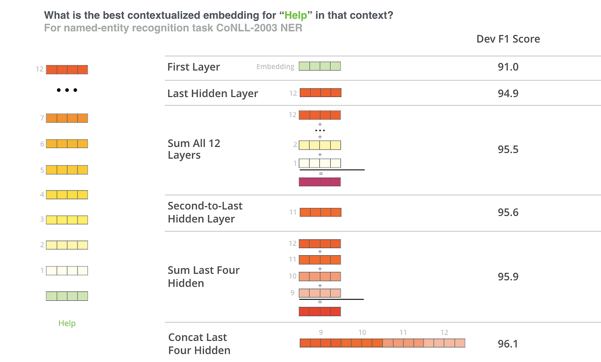
While concatenation of the last four layers produced the best results on this specific task, many of the other methods come in a close second and in general it is advisable to test different versions for your specific application: results may vary.
This is partially demonstrated by noting that the different layers of BERT encode very different kinds of information, so the appropriate pooling strategy will change depending on the application because different layers encode different kinds of information.
Han Xiao’s BERT-as-service
Han Xiao created an open-source project named bert-as-service on GitHub which is intended to create word embeddings for your text using BERT. Han experimented with different approaches to combining these embeddings, and shared some conclusions and rationale on the FAQ page of the project.
bert-as-service, by default, uses the outputs from the second-to-last layer of the model.
This is the summary of Han’s perspective :
- The embeddings start out in the first layer as having no contextual information (i.e., the meaning of the initial ‘bank’ embedding isn’t specific to river bank or financial bank).
- As the embeddings move deeper into the network, they pick up more and more contextual information with each layer.
- As you approach the final layer, however, you start picking up information that is specific to BERT’s pre-training tasks (the “Masked Language Model” (MLM) and “Next Sentence Prediction” (NSP)).
- What we want is embeddings that encode the word meaning well…
- BERT is motivated to do this, but it is also motivated to encode anything else that would help it determine what a missing word is (MLM), or whether the second sentence came after the first (NSP).
4. The second-to-last layer is what Han settled on as a reasonable sweet-spot.
- High-Dimensional:A BERT base model typically produces a 768-dimensional vector for each token.
Illustrative Understaing of Bert Model
Bidirectional encoder representations from transformers is a lanaguage model by Google , language model is an algorithm that predict missing word in a sequence(sentence). Our computers do not understand the English words or sentences they only understand the numbers. Bert are powerfull in generating the contextual(meaningful) vectors(number) representation of a given word, in technical term we call this process word embedding.
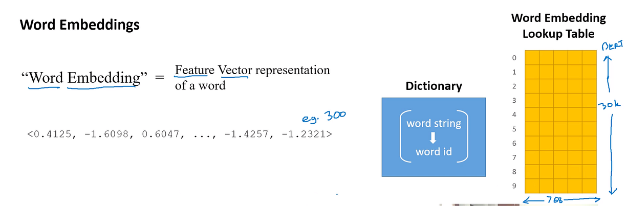
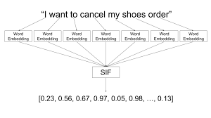
Word Embedding
Word embedding is a numerical representation of text(in the form of vectoe) where words with similar meanings have a similar representation.
I can generate the contextual embedding vector for the entire sentence.
ARCHITECTURE
Bert is based on transformer architecture. The Bert model is available in two sizes.
Get Sahil Kumar’s stories in your inbox
Join Medium for free to get updates from this writer.Subscribe
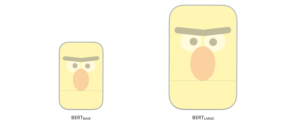
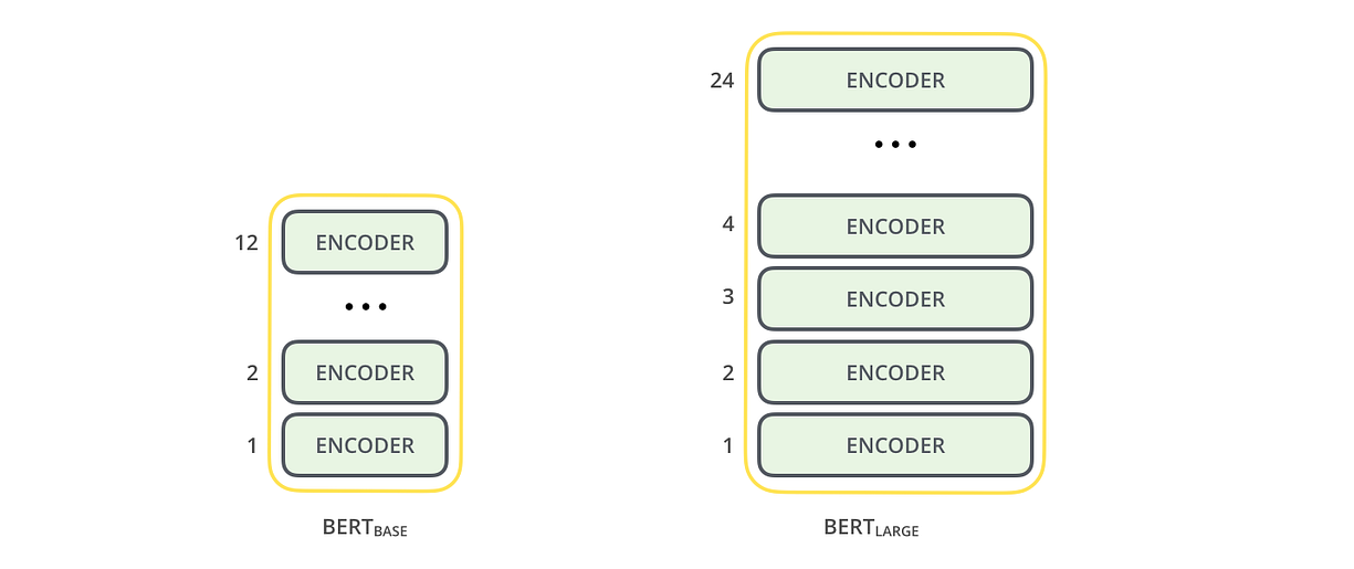
Bert base is small in size having 12 encoder layers and trained in 110M parameters on the other hand Bert large is larger and trained in 340M parameters.
Traning
Bert is trained by Google using two approches, 1. MLM (Masked language Model) 2. NSP (Next Sequence Prediction). In the first approch some words are masked (15% of the imput)

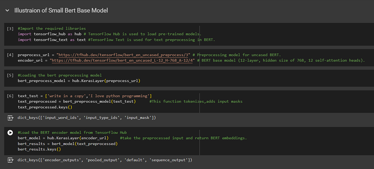
Illustration of Bert Base Model
Now I will be showing how to get the embedding vector for a sentence using the Bert base model.