𝐿𝑜𝑔𝑖𝑠𝑡𝑖𝑐 𝑟𝑒𝑔𝑟𝑒𝑠𝑠𝑖𝑜𝑛𝑝

(𝑦) =11+𝑒−(𝑏𝑜+𝑏1𝑥1+𝑏2𝑥2)

𝑆𝑡𝑒𝑝 − 1: 𝑋1 𝑎𝑛𝑑 𝑋2 𝑎𝑟𝑒 𝑝𝑎𝑠𝑠𝑖𝑛𝑔

𝑆𝑡𝑒𝑝 − 2: 𝑋1𝑖𝑠 𝑚𝑢𝑙𝑡𝑖𝑝𝑙𝑦 𝑤𝑖𝑡ℎ 𝑏1, 𝑋2 𝑚𝑢𝑙𝑡𝑖𝑝𝑙𝑒 𝑤𝑖𝑡ℎ 𝑏2

𝑆𝑡𝑒𝑝 − 3: 𝑏𝑜𝑖𝑠 𝑎𝑑𝑑𝑖𝑛𝑔𝑏𝑦 𝑡ℎ𝑖𝑠 𝑎 𝑒𝑞𝑢𝑎𝑡𝑖𝑜𝑛: 𝑦 = 𝑏𝑜 + 𝑏1* 𝑥1 + 𝑏2* 𝑥2

𝑆𝑡𝑒𝑝 − 4: 𝑡ℎ𝑒 𝑦 𝑖𝑠 𝑝𝑎𝑠𝑠𝑖𝑛𝑔 𝑡ℎ𝑟𝑜𝑢𝑔ℎ 𝐴𝑐𝑡𝑖𝑣𝑎𝑡𝑖𝑜𝑛 𝑓𝑢𝑛𝑐𝑡𝑖𝑜𝑛 𝑜𝑟 𝑠𝑖𝑔𝑚𝑜𝑖𝑑 𝑓𝑢𝑛𝑐𝑡𝑜𝑛σ(𝑦)

𝑆𝑡𝑒𝑝 − 5 = 𝑝(𝑦)𝑁𝑢𝑒𝑟𝑜𝑟𝑛:𝐷𝑒𝑒𝑝 𝑙𝑒𝑎𝑟𝑛𝑖𝑛𝑔 𝑐𝑜𝑛𝑠𝑖𝑡 𝑜𝑓 𝑁𝑢𝑒𝑟𝑜𝑛𝑠 𝑒𝑎𝑐ℎ 𝑛𝑒𝑢𝑟𝑜𝑛 𝑟𝑒𝑝𝑟𝑒𝑠𝑛𝑡𝑠 𝑤𝑖𝑡ℎ 𝑎 𝑟𝑜𝑢𝑛𝑑 𝑐𝑖𝑟𝑐𝑙𝑒𝐼𝑛 𝑒𝑎𝑐ℎ 𝑛𝑒𝑢𝑟𝑜𝑛 𝑡ℎ𝑒𝑟𝑒 𝑎𝑟𝑒 𝑡𝑤𝑜 𝑜𝑝𝑒𝑟𝑎𝑡𝑖𝑜𝑛𝑠

● 𝑠𝑢𝑚𝑚𝑎𝑡𝑖𝑜𝑛

● 𝐴𝑐𝑡𝑖𝑣𝑎𝑡𝑖𝑜𝑛ℎ2𝑜 = 𝑎𝑐𝑡𝑖𝑣𝑎𝑡𝑖𝑜𝑛(𝑤ℎ2 + 𝑤12* 𝑥1 + 𝑤22* 𝑥2 + 𝑤32* 𝑥3)

𝑇ℎ𝑟𝑒𝑒 𝑡𝑦𝑝𝑒𝑠 𝑜𝑓 𝑙𝑎𝑦𝑒𝑟𝑠 𝑎𝑣𝑎𝑖𝑙𝑎𝑏𝑙𝑒1) 𝐼𝑛𝑝𝑢𝑡 𝑙𝑎𝑦𝑒𝑟2) 𝐻𝑖𝑑𝑑𝑒𝑛 𝑙𝑎𝑦𝑒𝑟3) 𝑂𝑢𝑡𝑝𝑢𝑡 𝑙𝑎𝑦𝑒𝑟𝐼𝑛𝑝𝑢𝑡 𝑙𝑎𝑦𝑒𝑟

● 𝐼𝑛𝑝𝑢𝑡 𝑙𝑎𝑦𝑒𝑟 𝑖𝑠 𝑢𝑠𝑒𝑑 𝑡𝑜 𝑝𝑎𝑠𝑠 𝑡ℎ𝑒 𝑖𝑛𝑝𝑢𝑡𝑠

● 𝐼𝑛𝑝𝑢𝑡 𝑙𝑎𝑦𝑒𝑟 𝑐𝑜𝑛𝑠𝑖𝑠𝑡 𝑛𝑒𝑢𝑟𝑜𝑛𝑠

● 𝑇ℎ𝑒 𝑛𝑢𝑚𝑏𝑒𝑟 𝑜𝑓 𝑛𝑒𝑢𝑟𝑜𝑛𝑠 𝑒𝑞𝑢𝑎𝑙 𝑡𝑜 𝑛𝑢𝑚𝑏𝑒𝑟 𝑜𝑓 𝑖𝑛𝑝𝑢𝑡𝑠

● 𝐹𝑜𝑟 𝑒𝑥𝑎𝑚𝑝𝑙𝑒 𝑖𝑛 𝑤𝑖𝑛𝑒 𝑞𝑢𝑙𝑎𝑖𝑡𝑦 𝑑𝑎𝑡𝑠𝑒𝑡𝑠 𝑡ℎ𝑒 𝑛𝑢𝑚𝑏𝑒𝑟 𝑖𝑛𝑝𝑢𝑡𝑠 = 𝑛𝑢𝑚𝑏𝑒𝑟 𝑜𝑓 𝑐𝑜𝑙𝑢𝑚𝑛𝑠

● 𝑡ℎ𝑒𝑟𝑒 𝑎𝑟𝑒 11 𝑖𝑛𝑝𝑢𝑡 𝑐𝑜𝑙𝑢𝑚𝑛𝑠 𝑎𝑟𝑒 𝑡ℎ𝑒𝑟𝑒 𝑠𝑜 𝑤𝑒 ℎ𝑎𝑣𝑒 11 𝑛𝑒𝑢𝑟𝑜𝑛𝑠

● 𝐹𝑜𝑟 𝑒𝑥𝑎𝑚𝑝𝑙𝑒 𝑎𝑛 𝑖𝑚𝑎𝑔𝑒 𝑠𝑖𝑧𝑒 ℎ𝑎𝑠 28 * 28 = 784 𝑝𝑖𝑥𝑒𝑙𝑠 𝑤𝑒 ℎ𝑎𝑣𝑒

● 𝑠𝑜 𝑡ℎ𝑎𝑡 𝑤𝑒 𝑟𝑒𝑞𝑢𝑖𝑟𝑒𝑑 784 𝑛𝑒𝑢𝑟𝑜𝑛𝑠

● 𝐼𝑛𝑝𝑢𝑡 𝑛𝑒𝑢𝑟𝑜𝑛𝑠 𝑢𝑠𝑒𝑑 𝑜𝑛𝑙𝑦 𝑓𝑜𝑟 𝑝𝑎𝑠𝑠𝑖𝑛𝑔 𝑡ℎ𝑒 𝑖𝑛𝑝𝑢𝑡𝑠

● 𝑊ℎ𝑖𝑙𝑒 𝑝𝑎𝑠𝑠𝑖𝑛𝑔 𝑖𝑡 𝑤𝑖𝑙𝑙 𝑛𝑜𝑡 𝑚𝑢𝑙𝑡𝑖𝑝𝑙𝑦 𝑤𝑖𝑡ℎ 𝑎𝑛𝑦 𝑤𝑒𝑖𝑔ℎ𝑡𝑠

● 𝑆𝑜 𝑖𝑛 𝑡ℎ𝑒 𝑖𝑛𝑝𝑢𝑡 𝑛𝑒𝑢𝑟𝑜𝑛𝑠 𝑛𝑜 𝑠𝑢𝑚𝑚𝑎𝑡𝑖𝑜𝑛 𝑎𝑛𝑑 𝑛𝑜 𝑎𝑐𝑡𝑖𝑣𝑎𝑡𝑖𝑜𝑛𝐻𝑖𝑑𝑑𝑒𝑛 𝑙𝑎𝑦𝑒𝑟𝑠

● 𝐻𝑖𝑑𝑑𝑒𝑛 𝑙𝑎𝑦𝑒𝑟𝑠 𝑎𝑟𝑒 𝑏𝑒𝑡𝑤𝑒𝑒𝑛 𝑖𝑛𝑝𝑢𝑡 𝑎𝑛𝑑 𝑜𝑢𝑡𝑝𝑢𝑡 𝑙𝑎𝑦𝑒𝑟

● 𝐼𝑡 𝑖𝑠 𝑐𝑎𝑙𝑙𝑒𝑑 ℎ𝑖𝑑𝑑𝑒𝑛 𝑏𝑒𝑐𝑎𝑢𝑠𝑒 𝑖𝑡 𝑑𝑜𝑒𝑠 𝑛𝑜𝑡 𝑡𝑎𝑘𝑒𝑠 𝑡ℎ𝑒 𝑖𝑛𝑝𝑢𝑡𝑠 𝑑𝑖𝑟𝑒𝑐𝑡𝑙𝑦

● 𝑇ℎ𝑒 𝑖𝑛𝑝𝑢𝑡 𝑣𝑎𝑙𝑢𝑒 𝑓𝑜𝑟 ℎ𝑖𝑑𝑑𝑒𝑛 𝑙𝑎𝑦𝑒𝑟 𝑖𝑠: 𝑖𝑛𝑝𝑢𝑡 𝑑𝑎𝑡𝑎 𝑚𝑢𝑙𝑡𝑖𝑝𝑙𝑦 𝑤𝑖𝑡ℎ 𝑤𝑒𝑖𝑔ℎ𝑡

● ℎ𝑖𝑑𝑑𝑒𝑛 𝑙𝑎𝑦𝑒𝑟𝑠 𝑎𝑟𝑒 𝑢𝑠𝑒𝑑 𝑡𝑜 𝑖𝑑𝑒𝑛𝑡𝑖𝑓𝑦 𝑡ℎ𝑒 𝑝𝑎𝑡𝑡𝑒𝑟𝑛𝑠𝑂𝑢𝑡𝑝𝑢𝑡 𝑙𝑎𝑦𝑒𝑟

● 𝑂𝑢𝑡𝑝𝑢𝑡 𝑙𝑎𝑦𝑒𝑟 𝑖𝑠 𝑢𝑠𝑒𝑑 𝑡𝑜 𝑝𝑟𝑜𝑣𝑖𝑑𝑒 𝑜𝑢𝑡𝑝𝑢𝑡𝑠

● 𝐵𝑖 𝑐𝑙𝑎𝑠𝑠𝑖𝑓𝑖𝑐𝑎𝑡𝑖𝑜𝑛 : 𝑂𝑛𝑒 𝑛𝑒𝑢𝑟𝑜𝑛

● 𝑀𝑢𝑙𝑡𝑖 𝑐𝑙𝑎𝑠𝑠𝑖𝑓𝑖𝑐𝑎𝑡𝑖𝑜𝑛: 𝑀𝑢𝑙𝑡𝑖𝑝𝑙𝑒 𝑛𝑒𝑢𝑟𝑜𝑛𝑠

● 10 𝑐𝑙𝑎𝑠𝑠𝑒𝑠 : 10 𝑛𝑒𝑢𝑟𝑜𝑛𝑠

● 𝐸𝑎𝑐ℎ 𝑛𝑒𝑢𝑟𝑜𝑛 ℎ𝑎𝑠 𝑏𝑖𝑎𝑠 𝑎𝑛𝑑 𝑤𝑒𝑖𝑔ℎ𝑡𝑠𝐷𝑒𝑒𝑝 𝑙𝑒𝑎𝑟𝑛𝑖𝑛𝑔𝑇𝑦𝑝𝑒𝑠 𝑜𝑓 𝐺𝑎𝑟𝑑𝑖𝑒𝑛𝑡 𝑑𝑒𝑠𝑐𝑒𝑛𝑡𝑀𝑒𝑡𝑟𝑖𝑐𝑠 𝑖𝑛 𝐷𝐿 𝑖𝑠 𝑠𝑎𝑚𝑒 𝑎𝑠 𝐶𝑙𝑎𝑠𝑠𝑖𝑓𝑖𝑐𝑎𝑡𝑖𝑜𝑛 𝑚𝑒𝑡𝑟𝑖𝑐𝑠 𝑖. 𝑒 𝑎𝑐𝑐𝑢𝑎𝑟𝑐𝑦 , 𝑝𝑟𝑒𝑐𝑠𝑖𝑜𝑛, 𝑟𝑒𝑐𝑎𝑙𝑙 𝑓1𝑠𝑐𝑜𝑟𝑒𝐵𝑢𝑡 𝑖𝑛 𝑑𝑒𝑒𝑝 𝑙𝑒𝑎𝑟𝑛𝑖𝑛𝑔 𝑤𝑒 𝑢𝑠𝑒 𝑜𝑛𝑒 𝑚𝑜𝑟𝑒 𝑚𝑒𝑡𝑟𝑖𝑐 𝑙𝑜𝑠𝑠 𝑓𝑢𝑛𝑐𝑡𝑖𝑜𝑛𝐿𝑜𝑠𝑠 𝑓𝑢𝑛𝑐𝑡𝑖𝑜𝑛:

● 𝐵𝑖𝑛𝑎𝑟𝑦 𝑐𝑟𝑜𝑠𝑠 𝑒𝑛𝑡𝑟𝑜𝑝𝑦 : 𝐵𝑖 𝑐𝑙𝑎𝑠𝑠𝑖𝑓𝑖𝑐𝑎𝑡𝑖𝑜𝑛

● 𝑆𝑝𝑎𝑟𝑠𝑒 𝑐𝑎𝑡𝑒𝑔𝑜𝑟𝑖𝑐𝑎𝑙 𝑐𝑟𝑜𝑠𝑠 𝑒𝑛𝑡𝑟𝑜𝑝𝑦 : 𝑀𝑢𝑙𝑡𝑖 𝑐𝑙𝑎𝑠𝑠𝑖𝑓𝑖𝑐𝑎𝑡𝑖𝑜𝑛𝐶𝑟𝑜𝑠𝑠 𝑒𝑛𝑡𝑟𝑜𝑝𝑦:𝐸𝑛𝑡𝑟𝑜𝑝𝑦 = − 𝑝𝑦𝑒𝑠* 𝑙𝑜𝑔𝑝𝑦𝑒𝑠 − 𝑝𝑛𝑜* 𝑙𝑜𝑔 𝑝 𝑛𝑜 = 1 − 𝑝𝑦𝑒𝑠( )𝐶𝑟𝑜𝑠𝑠 𝐸𝑛𝑡𝑟𝑜𝑝𝑦 = − 𝑝𝑦𝑒𝑠* 𝑙𝑜𝑔𝑝𝑦𝑒𝑠 − 1 − 𝑝𝑦𝑒𝑠( ) * 𝑙𝑜𝑔 1 − 𝑝𝑦𝑒𝑠( )

● 𝐺𝑒𝑛𝑒𝑟𝑎𝑙𝑙𝑦 𝑂𝑢𝑡𝑝𝑢𝑡 𝑛𝑒𝑡𝑤𝑜𝑟𝑘 𝑝𝑟𝑜𝑣𝑖𝑑𝑒𝑠 𝑠𝑜𝑚𝑒 𝑣𝑎𝑙𝑢𝑒𝑠 (𝑙𝑜𝑔𝑖𝑡𝑠), = 𝑊 * 𝑋 + 𝑏

● 𝑡ℎ𝑎𝑡 𝑣𝑎𝑙𝑢𝑒𝑠 𝑝𝑎𝑠𝑠 𝑡ℎ𝑟𝑜𝑢𝑔ℎ 𝑎𝑐𝑡𝑖𝑣𝑎𝑡𝑖𝑜𝑛 𝑓𝑢𝑛𝑐𝑡𝑖𝑜𝑛 (𝑝𝑟𝑜𝑏𝑎𝑏𝑖𝑙𝑡𝑖𝑒𝑠) = 𝑠𝑖𝑔𝑚𝑜𝑖𝑑(𝑊 * 𝑋 + 𝑏)

● 𝑎𝑐𝑡𝑖𝑣𝑎𝑡𝑖𝑜𝑛 𝑓𝑢𝑛𝑐𝑡𝑖𝑜𝑛 𝑐𝑜𝑛𝑣𝑒𝑟𝑡𝑠 𝑡ℎ𝑜𝑠𝑒 𝑣𝑎𝑙𝑢𝑒𝑠 𝑖𝑛𝑡𝑜 𝑝𝑟𝑜𝑏𝑎𝑏𝑖𝑙𝑡𝑦 𝑣𝑎𝑙𝑢𝑒𝑠

● 𝑤ℎ𝑖𝑐ℎ 𝑒𝑣𝑒𝑟 𝑖𝑠 𝑡ℎ𝑒 ℎ𝑖𝑔ℎ𝑒𝑠𝑡 𝑝𝑟𝑜𝑏𝑎𝑏𝑖𝑙𝑖𝑡𝑦 𝑡ℎ𝑎𝑡 𝑏𝑒𝑐𝑜𝑚𝑒𝑠 𝑡ℎ𝑒 𝑜𝑢𝑡𝑝𝑢𝑡𝐴𝑠𝑠𝑢𝑚𝑒 𝑡ℎ𝑎𝑡 𝑤𝑒 𝑤𝑎𝑛𝑡 𝑝𝑒𝑟𝑓𝑜𝑟𝑚 𝑎𝑛𝑖𝑚𝑎𝑙 𝑜𝑏𝑗𝑒𝑐𝑡 𝑑𝑒𝑡𝑒𝑐𝑡𝑖𝑜𝑛𝑇ℎ𝑒𝑟𝑒 𝑎𝑟𝑒 3 𝑐𝑙𝑎𝑠𝑠𝑒𝑠 𝑎𝑟𝑒 𝑡ℎ𝑒𝑟𝑒

● 𝐷𝑜𝑔

● 𝐶𝑎𝑡

● 𝑅𝑎𝑏𝑏𝑖𝑡

𝑊𝑒 𝑎𝑟𝑒 𝑝𝑎𝑠𝑠𝑖𝑛𝑔 𝐷𝑜𝑔 𝑖𝑚𝑎𝑔𝑒 𝑡𝑜 𝑡ℎ𝑒 𝑁𝑒𝑢𝑟𝑎𝑙 𝑛𝑒𝑡𝑤𝑜𝑟𝑘𝑇ℎ𝑒𝑟𝑒 𝑎𝑟𝑒 3 𝑐𝑜𝑚𝑏𝑖𝑛𝑎𝑡𝑖𝑜𝑛𝑠𝐴𝑐𝑡𝑢𝑎𝑙𝑙𝑦 𝐷𝑜𝑔 , 𝑁𝑒𝑡𝑤𝑜𝑟𝑘 𝑝𝑟𝑒𝑑𝑖𝑐𝑡𝑒𝑑 𝑎𝑠 𝐷𝑜𝑔𝐴𝑐𝑡𝑢𝑎𝑙𝑙𝑦 𝐷𝑜𝑔 , 𝑁𝑒𝑡𝑤𝑜𝑟𝑘 𝑝𝑟𝑒𝑑𝑖𝑐𝑡𝑒𝑑 𝑎𝑠 𝐶𝑎𝑡𝐴𝑐𝑡𝑢𝑎𝑙𝑙𝑦 𝐷𝑜𝑔 , 𝑁𝑒𝑡𝑤𝑜𝑟𝑘 𝑝𝑟𝑒𝑑𝑖𝑐𝑡𝑒𝑑 𝑎𝑠 𝑅𝑎𝑏𝑏𝑖𝑡𝑀𝑒𝑡𝑟𝑖𝑐𝑠 𝑖𝑛 𝐷𝐿 𝑖𝑠 𝑠𝑎𝑚𝑒 𝑎𝑠 𝐶𝑙𝑎𝑠𝑠𝑖𝑓𝑖𝑐𝑎𝑡𝑖𝑜𝑛 𝑚𝑒𝑡𝑟𝑖𝑐𝑠 𝑖. 𝑒 𝑎𝑐𝑐𝑢𝑎𝑟𝑐𝑦 , 𝑝𝑟𝑒𝑐𝑠𝑖𝑜𝑛, 𝑟𝑒𝑐𝑎𝑙𝑙 𝑓1𝑠𝑐𝑜𝑟𝑒𝐵𝑢𝑡 𝑖𝑛 𝑑𝑒𝑒𝑝 𝑙𝑒𝑎𝑟𝑛𝑖𝑛𝑔 𝑤𝑒 𝑢𝑠𝑒 𝑜𝑛𝑒 𝑚𝑜𝑟𝑒 𝑚𝑒𝑡𝑟𝑖𝑐 𝑙𝑜𝑠𝑠 𝑓𝑢𝑛𝑐𝑡𝑖𝑜𝑛𝐿𝑜𝑠𝑠 𝑓𝑢𝑛𝑐𝑡𝑖𝑜𝑛:

● 𝐵𝑖𝑛𝑎𝑟𝑦 𝑐𝑟𝑜𝑠𝑠 𝑒𝑛𝑡𝑟𝑜𝑝𝑦 : 𝐵𝑖 𝑐𝑙𝑎𝑠𝑠𝑖𝑓𝑖𝑐𝑎𝑡𝑖𝑜𝑛

● 𝑆𝑝𝑎𝑟𝑠𝑒 𝑐𝑎𝑡𝑒𝑔𝑜𝑟𝑖𝑐𝑎𝑙 𝑐𝑟𝑜𝑠𝑠 𝑒𝑛𝑡𝑟𝑜𝑝𝑦 : 𝑀𝑢𝑙𝑡𝑖 𝑐𝑙𝑎𝑠𝑠𝑖𝑓𝑖𝑐𝑎𝑡𝑖𝑜𝑛𝐶𝑟𝑜𝑠𝑠 𝑒𝑛𝑡𝑟𝑜𝑝𝑦:𝐸𝑛𝑡𝑟𝑜𝑝𝑦 = − 𝑝𝑦𝑒𝑠* 𝑙𝑜𝑔𝑝𝑦𝑒𝑠 − 𝑝𝑛𝑜* 𝑙𝑜𝑔 𝑝 𝑛𝑜 = 1 − 𝑝𝑦𝑒𝑠( )𝐶𝑟𝑜𝑠𝑠 𝐸𝑛𝑡𝑟𝑜𝑝𝑦 = − 𝑝𝑦𝑒𝑠* 𝑙𝑜𝑔𝑝𝑦𝑒𝑠 − 1 − 𝑝𝑦𝑒𝑠( ) * 𝑙𝑜𝑔 1 − 𝑝𝑦𝑒𝑠( )

● 𝐺𝑒𝑛𝑒𝑟𝑎𝑙𝑙𝑦 𝑂𝑢𝑡𝑝𝑢𝑡 𝑛𝑒𝑡𝑤𝑜𝑟𝑘 𝑝𝑟𝑜𝑣𝑖𝑑𝑒𝑠 𝑠𝑜𝑚𝑒 𝑣𝑎𝑙𝑢𝑒𝑠 (𝑙𝑜𝑔𝑖𝑡𝑠), = 𝑊 * 𝑋 + 𝑏

● 𝑡ℎ𝑎𝑡 𝑣𝑎𝑙𝑢𝑒𝑠 𝑝𝑎𝑠𝑠 𝑡ℎ𝑟𝑜𝑢𝑔ℎ 𝑎𝑐𝑡𝑖𝑣𝑎𝑡𝑖𝑜𝑛 𝑓𝑢𝑛𝑐𝑡𝑖𝑜𝑛 (𝑝𝑟𝑜𝑏𝑎𝑏𝑖𝑙𝑡𝑖𝑒𝑠) = 𝑠𝑖𝑔𝑚𝑜𝑖𝑑(𝑊 * 𝑋 + 𝑏)

● 𝑎𝑐𝑡𝑖𝑣𝑎𝑡𝑖𝑜𝑛 𝑓𝑢𝑛𝑐𝑡𝑖𝑜𝑛 𝑐𝑜𝑛𝑣𝑒𝑟𝑡𝑠 𝑡ℎ𝑜𝑠𝑒 𝑣𝑎𝑙𝑢𝑒𝑠 𝑖𝑛𝑡𝑜 𝑝𝑟𝑜𝑏𝑎𝑏𝑖𝑙𝑡𝑦 𝑣𝑎𝑙𝑢𝑒𝑠

● 𝐼𝑓 𝑀𝑜𝑑𝑒𝑙 𝑤𝑖𝑙𝑙 𝑐𝑙𝑒𝑎𝑟𝑙𝑦 𝐷𝑖𝑠𝑐𝑟𝑖𝑚𝑖𝑛𝑎𝑡𝑒 𝑡ℎ𝑒 𝑙𝑎𝑏𝑙𝑒𝑠 𝑤𝑖𝑡ℎ 𝑝𝑟𝑜𝑏𝑎𝑏𝑖𝑙𝑡𝑖𝑒𝑠 𝑡ℎ𝑒𝑛 𝐶𝑟𝑜𝑠𝑠 𝑒𝑛𝑡𝑟𝑜𝑝 𝑙𝑜𝑤

● 𝐼𝑓 𝑀𝑜𝑑𝑒𝑙 𝑤𝑖𝑙𝑙 𝑝𝑟𝑒𝑑𝑖𝑐𝑡 𝑐𝑜𝑟𝑟𝑒𝑐𝑡 𝑎𝑛𝑠𝑤𝑒𝑟𝑠 𝑏𝑢𝑡 𝑡ℎ𝑒 𝑝𝑟𝑜𝑏𝑎𝑏𝑖𝑙𝑡𝑖𝑒𝑠 𝑎𝑟𝑒 𝑛𝑜𝑡 𝑚𝑢𝑐ℎ 𝑑𝑖𝑓𝑓𝑒𝑟 𝑡ℎ𝑒𝑛 𝐶𝐸 ℎ𝑖𝑔ℎ

● 𝐼𝑓 𝑚𝑜𝑑𝑒𝑙 𝑝𝑟𝑒𝑑𝑖𝑐𝑡𝑠 𝑤𝑟𝑜𝑛𝑔 𝑎𝑛𝑠𝑤𝑒𝑟 𝑡ℎ𝑒𝑛 𝐶𝑟𝑜𝑠𝑠 𝑒𝑛𝑡𝑟𝑜𝑝 𝑤𝑖𝑙𝑙 𝑏𝑒 𝐻𝑢𝑔𝑒

● 𝐴𝑐𝑐𝑢𝑟𝑎𝑐𝑦 𝑤𝑖𝑙𝑙 𝑡𝑒𝑙𝑙 𝑡ℎ𝑒 𝑐𝑜𝑟𝑟𝑒𝑐𝑡 𝑝𝑟𝑒𝑑𝑖𝑐𝑡𝑖𝑜𝑛𝑠 𝑤𝑖𝑡ℎ 𝑜𝑢𝑡 𝑟𝑒𝑙𝑎𝑡𝑒𝑑 𝑡𝑜 𝑚𝑜𝑑𝑒𝑙 𝑐𝑜𝑛𝑓𝑖𝑑𝑒𝑛𝑐𝑒

● 𝐶𝑟𝑜𝑠𝑠 𝑒𝑛𝑡𝑟𝑜𝑝𝑦 𝑤𝑖𝑙𝑙 𝑔𝑖𝑣𝑒 𝑡ℎ𝑒 𝑖𝑑𝑒𝑎 ℎ𝑜𝑤 𝑚𝑢𝑐ℎ 𝑜𝑢𝑟 𝑚𝑜𝑑𝑒𝑙 𝑐𝑜𝑛𝑓𝑖𝑑𝑒𝑛𝑡𝑂𝑝𝑡𝑖𝑚𝑖𝑧𝑒𝑟𝐼𝑠 𝑢𝑠𝑒𝑑 𝑡𝑜 𝑠𝑝𝑒𝑒𝑑 𝑢𝑝 𝑡ℎ𝑒 𝑝𝑟𝑜𝑐𝑒𝑠𝑠 𝑡𝑜 𝑓𝑖𝑛𝑑 𝑡ℎ𝑒 𝑤𝑒𝑖𝑔ℎ𝑡𝑠𝐺𝑒𝑛𝑒𝑟𝑎𝑙𝑙𝑦 𝑡𝑜 𝑓𝑖𝑛𝑑 𝑡ℎ𝑒 𝑤𝑒𝑖𝑔ℎ𝑡𝑠 𝑤𝑒 ℎ𝑎𝑣𝑒 𝐺𝑟𝑑𝑖𝑒𝑛𝑡 𝑑𝑒𝑠𝑐𝑒𝑛𝑡 𝑤𝑖𝑙𝑙 𝑢𝑠𝑒𝐵𝑢𝑡 𝑔𝑟𝑎𝑑𝑖𝑒𝑛𝑡 𝑑𝑒𝑠𝑐𝑒𝑛𝑡 𝑓𝑎𝑖𝑙 𝑤ℎ𝑒𝑛 𝑤𝑒 ℎ𝑎𝑣𝑒 𝑡𝑤𝑜 𝑚𝑖𝑛𝑚𝑢𝑚 𝑝𝑜𝑖𝑛𝑡𝑠𝑙𝑜𝑐𝑎𝑙 𝑚𝑖𝑛𝑖𝑚𝑎 𝑎𝑛𝑑 𝐺𝑙𝑜𝑏𝑎𝑙 𝑚𝑖𝑛𝑖𝑚𝑎𝐺𝑟𝑎𝑑𝑖𝑒𝑛𝑡 𝑑𝑒𝑠𝑐𝑒𝑛𝑡𝐺𝑟𝑎𝑑𝑖𝑒𝑛𝑡 𝑑𝑒𝑠𝑐𝑒𝑛𝑡 𝑤𝑖𝑡ℎ 𝑀𝑜𝑚𝑒𝑛𝑡𝑢𝑚 : 𝐺𝑙𝑜𝑏𝑎𝑙 𝑚𝑖𝑛𝑖𝑚𝑎𝐴𝑑𝑎𝑝𝑡𝑖𝑣𝑒 𝐺𝑟𝑎𝑑𝑖𝑒𝑛𝑡 𝑑𝑒𝑠𝑐𝑒𝑛𝑡 : 𝐿𝑒𝑎𝑟𝑛𝑖𝑛 𝑟𝑎𝑡𝑒𝑅𝑚𝑠 𝑃𝑟𝑜𝑝 : 𝐷𝑒𝑐𝑎𝑦 𝑟𝑎𝑡𝑒 (𝑀𝑜𝑚𝑒𝑛𝑡𝑢𝑚)𝐴𝑑𝑎𝑚 (𝐴𝑑𝐺𝑟𝑎𝑑𝑒 + 𝑅𝑚𝑠𝑃𝑟𝑜𝑝)

An Artificial Neural Network (ANN) is a computational model inspired by the human brain’s network of neurons. It consists of interconnected nodes called artificial neurons organized in layers: an input layer, one or more hidden layers, and an output layer. These neurons process input data by applying weights to connections and using nonlinear activation functions to produce outputs. Through a training process, the network adjusts these weights to minimize errors between predicted and actual results, enabling it to learn patterns and make predictions.ANNs are widely used in machine learning and artificial intelligence for tasks such as image and speech recognition, natural language processing, and forecasting. They can learn from experience by training on example data and improve their accuracy over time. Different architectures like feedforward, recurrent, and convolutional neural networks serve specific purposes depending on the problem type. This adaptive learning and pattern recognition make ANNs powerful tools across various domains.In summary, Artificial Neural Networks mimic brain-like learning to process complex data inputs and make intelligent decisions or predictions.

Differences between feedforward and recurrent neural networks

The primary differences between feedforward neural networks (FNNs) and recurrent neural networks (RNNs) are as follows:

Feature	Feedforward Neural Networks (FNN)	Recurrent Neural Networks (RNN)
Data Flow	One-way, from input to output, no cycles or loops	Cyclic, with loops allowing information to persist
Memory	No memory of previous inputs	Has internal memory via hidden states
Input Type	Best suited for static, fixed-size input data	Ideal for sequential or time-dependent data
Application Examples	Image classification, object detection	Language modeling, speech recognition, time series
Training Complexity	Simpler, faster to train	More complex, slower due to sequential dependencies
Training Challenges	Less prone to vanishing gradients	Can suffer from vanishing or exploding gradient problems
Processing Style	Inputs processed independently	Sequential processing with context from previous inputs
Handling Variable Length	Cannot handle variable-length input without preprocessing	Naturally processes variable-length sequences

FNNs process data in a single direction without feedback, making them effective for tasks where each input is independent, like static image data. RNNs, with their loops and memory mechanism, can retain context and are designed for sequential data where the order matters, such as language or time series analysis. However, RNNs are more computationally intensive and harder to train compared to FNNs.

An artificial neural network is a biologically inspired computational model that is patterned after the network of neurons present in the human brain. Artificial neural networks can also be thought of as learning algorithms that model the input-output relationship. Applications of artificial neural networks include pattern recognition and forecasting in fields such as medicine, business, pure sciences, data mining, telecommunications, and operations managements.

An artificial neural network transforms input data by applying a nonlinear function to a weighted sum of the inputs. The transformation is known as a neural layer and the function is referred to as a neural unit. The intermediate outputs of one layer, called features, are used as the input into the next layer. The neural network through repeated transformations learns multiple layers of nonlinear features (like edges and shapes), which it then combines in a final layer to create a prediction (of more complex objects). The neural net learns by varying the weights or parameters of a network so as to minimize the difference between the predictions of the neural network and the desired values. This phase where the artificial neural network learns from the data is called training.

Figure 1: : Schematic representation of a neural network

Neural networks where information is only fed forward from one layer to the next are called feedforward neural networks. On the other hand, the class of networks that has memory or feedback loops is called Recurrent Neural Networks.

Neural Network Inference

Once the artificial neural network has been trained, it can accurately predict outputs when presented with inputs, a process referred to as neural network inference. To perform inference, the trained neural network can be deployed in platforms ranging from the cloud, to enterprise datacenters, to resource-constrained edge devices. The deployment platform and type of application impose unique latency, throughput, and application size requirements on runtime. For example, a neural network performing lane detection in a car needs to have low latency and a small runtime application. On the other hand, datacenter identifying objects in video streams needs to process thousands of video streams simultaneously, needing high throughput and efficiency.

Neural Network Terminology

UNIT

A unit often refers to a nonlinear activation function (such as the logistic sigmoid function) in a neural network layer that transforms the input data. The units in the input/ hidden/ output layers are referred to as input/ hidden/ output units. A unit typically has multiple incoming and outgoing connections. Complex units such as long short-term memory (LSTM) units have multiple activation functions with a distinct layout of connections to the nonlinear activation functions, or maxout units, which compute the final output over an array of nonlinearly transformed input values. Pooling, convolution, and other input transforming functions are usually not referred to as units.

ARTIFICIAL NEURON

The terms neuron or artificial neuron are equivalent to a unit, but imply a close connection to a biological neuron. However, deep learning does not have much to do with neurobiology and the human brain. On a micro level, the term neuron is used to explain deep learning as a mimicry of the human brain. On a macro level, Artificial Intelligence can be thought of as the simulation of human level intelligence using machines. Biological neurons are however now believed to be more similar to entire multilayer perceptrons than to a single unit/ artificial neuron in a neural network. Connectionist models of human perception and cognition utilize artificial neural networks. These connectionist models of the brain as neural nets formed of neurons and their synapses are different from the classical view (computationalism) that human cognition is more similar to symbolic computation in digital computers. Relational Networks and Neural Turing Machines are provided as evidence that cognition models of connectionism and computationalism need not be at odds and can coexist.

ACTIVATION FUNCTION

An activation function, or transfer function, applies a transformation on weighted input data (matrix multiplication between input data and weights). The function can be either linear or nonlinear. Units differ from transfer functions in their increased level of complexity. A unit can have multiple transfer functions (LSTM units) or a more complex structure (maxout units).

The features of 1000 layers of pure linear transformations can be reproduced by a single layer (because a chain of matrix multiplication can always be represented by a single matrix multiplication). A non-linear transformation, however, can create new, increasingly complex relationships. These functions are therefore very important in deep learning, to create increasingly complex features with every layer. Examples of nonlinear activation functions include logistic sigmoid, Tanh, and ReLU functions.

LAYER

A layer is the highest-level building block in machine learning. The first, middle, and last layers of a neural network are called the input layer, hidden layer, and output layer respectively. The term hidden layer comes from its output not being visible, or hidden, as a network output. A simple three-layer neural net has one hidden layer while the term deep neural net implies multiple hidden layers. Each neural layer contains neurons, or nodes, and the nodes of one layer are connected to those of the next. The connections between nodes are associated with weights that are dependent on the relationship between the nodes. The weights are adjusted so as to minimize the cost function by back-propagating the errors through the layers. The cost function is a measure of how close the output of the neural network algorithm is to the expected output. The error backpropagation to minimize the cost is done using optimization algorithms such as stochastic gradient descent, batch gradient descent, or mini-batch gradient descent algorithms. Stochastic gradient descent is a statistical approximation of the optimal change in gradient that produces the cost minima. The rate of change of the weights in the direction of the gradient is referred to as the learning rate. A low learning rate corresponds to slower/ more reliable training while a high rate corresponds to quicker/ less reliable training that might not converge on an optimal solution.

A layer is a container that usually receives weighted input, transforms it with a set of mostly nonlinear functions and then passes these values as output to the next layer in the neural net. A layer is usually uniform, that is it only contains one type of activation function, pooling, convolution etc. so that it can be easily compared to other parts of the neural network.

Accelerating Artificial Neural Networks with GPUs

State-of-the-art Neural Networks can have from millions to well over one billion parameters to adjust via back-propagation. They also require a large amount of training data to achieve high accuracy, meaning hundreds of thousands to millions of input samples will have to be run through both a forward and backward pass. Because neural nets are created from large numbers of identical neurons they are highly parallel by nature. This parallelism maps naturally to GPUs, which provide a significant computation speed-up over CPU-only training.

GPUs have become the platform of choice for training large, complex Neural Network-based systems because of their ability to accelerate the systems. Because of the increasing importance of Neural networks in both industry and academia and the key role of GPUs, NVIDIA has a library of primitives called cuDNN that makes it easy to obtain state-of-the-art performance with Deep Neural Networks.

The parallel nature of inference operations also lend themselves well for execution on GPUs. To optimize, validate, and deploy networks for inference, NVIDIA has an inference platform accelerator and runtime called TensorRT. TensorRT delivers low-latency, high-throughput inference and tunes the runtime application to run optimally across different families of GPUs.

Understanding how neural networks are built is becoming more important as AI research grows. Two main types of structures—feedforward and (recurrent) neural networks—offer different ways of handling information. Neural networks are the backbone of many modern artificial intelligence systems, but not all neural networks are built the same. Two important types are feedforward and or recurrent neural networks.

While both are designed to process information and recognize patterns, they differ significantly in how data moves through them and the types of problems they are best suited to solve. In a feedforward network, information moves in one direction — from input to output — without any loops. These networks are great for tasks like image recognition and basic predictions.

networks, on the other hand, have loops that let them remember past information, making them perfect for things like understanding speech or analyzing time-based data. Knowing the difference between these two types helps us choose the right model for different kinds of AI problems.

In this article, we’ll break down both types, explain how they work, and compare their performance through simple examples and real-world use cases.

Prerequisites

Before diving into this article, it will help if you have:

• A basic understanding of how neural networks work.
• Familiarity with terms like neurons, layers, inputs, and outputs.
• A general idea of machine learning and AI concepts.

First, let’s start with the basics.

What is a Neural Network?

The fundamental building block of deep learning, a neural network is a computational model used to recognize patterns and make predictions or decisions based on data. The main inspiration behind this is the way the human brain functions, it consists of layers of neurons (also called nodes) connected by synapses. These neurons work together to process data and learn from it in a way that allows the network to improve its performance over time.

The structure of a neural network typically includes three main components:

1. Input Layer:
   • This is where the neural network receives data.
   • Each neuron in the input layer represents one feature or piece of information from the data. For example, in an image classification task, the pixels of an image could be the features input into the network.
2. Hidden Layers:
   • These layers sit between the input and output layers and do most of the computation.
   • Each neuron in a hidden layer takes input from the neurons of the previous layer, processes the data using mathematical functions, and passes the result to the next layer.
   • Hidden layers allow the network to learn complex patterns and relationships in the data. The more hidden layers there are, the deeper the network becomes, allowing it to capture intricate features of the data.
3. Output Layer:
   • The final layer of the neural network is where the processed data is transformed into a prediction or classification result.
   • For example, in a classification task, the output layer might give the probability of the input data belonging to each class.

The learning process in a neural network involves adjusting the weights of the connections between neurons in order to reduce the difference between the network’s output and the actual result (the error or loss).

How Does a Neural Network Learn?

Let us discuss the working of the neural network:

• Forward Propagation:
  • The data is passed through the network, starting from the input layer, moving through the hidden layers, and finally reaching the output layer. This is called forward propagation.
  • In each layer, the neurons perform mathematical operations, often using a function called an activation function to introduce non-linearity to the network. This helps the network learn complex patterns that are not just linear combinations of the input.
• Backpropagation:
  • After the output is generated, the network compares it to the correct output (the target) and calculates the error.
  • Backpropagation is the process of sending the error back through the network to adjust the weights of the connections between neurons. The goal is to reduce this error over time, which is done using optimization algorithms like gradient descent.
  • This process is repeated many times during training, with the weights being adjusted slightly each time, until the network is able to make predictions that are accurate enough for the task.

Elements of Neural Networks

The neurons that make up the neural network architecture replicate the organic behavior of the brain.

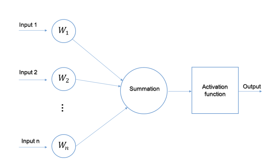
Elementary structure of a single neuron in a Neural Network

Now, we will define the various components related to the neural network and show how we can, starting from this basic representation of a neuron, build some of the most complex architectures.

Input

It is the collection of data (i.e, features) that is input into the learning model. For instance, an array of current atmospheric measurements can be used as the input for a meteorological prediction model.

Weight

Giving importance to features that help the learning process the most is the primary purpose of using weights. By adding scalar multiplication between the input value and the weight matrix, we can increase the effect of some features while lowering it for others. For instance, the presence of a high pitch note would influence the music genre classification model’s choice more than other average pitch notes that are common between genres.

Activation Function

In order to take into account changing linearity with the inputs, the activation function introduces non-linearity into the operation of neurons. Without it, the output would simply be a linear combination of the input values, and the network would not be able to accommodate non-linearity.

The most commonly used activation functions are: Unit step, sigmoid, piecewise linear, and Gaussian.

Illustrations of the common activation functions

Bias

The purpose of bias is to change the value that the activation function generates. Its function is comparable to a constant in a linear function. So, it’s a shift for the activation function output.

Layers

An artificial neural network is made of multiple neural layers stacked on top of one another. Each layer consists of several neurons stacked in a row. We distinguish three types of layers: Input, hidden, and Output.

Input Layer

The input layer of the model receives the data that we introduce to it from external sources like images or a numerical vector. It is the only layer that can be seen in the entire design of a neural network that transmits all of the information from the outside world without any processing.

Hidden Layers

The hidden layers are what make deep learning what it is today. They are intermediary layers that do all the calculations and extract the features of the data. The search for hidden features in data may comprise many interlinked hidden layers. In image processing, for example, the first hidden layers are often in charge of higher-level functions such as the detection of borders, shapes, and boundaries. The later hidden layers, on the other hand, perform more sophisticated tasks, such as classifying or segmenting entire objects.

Output Layer

The final prediction is made by the output layer using data from the preceding hidden layers. It is the layer from which we acquire the final result, hence it is the most important.

In the output layer, classification and regression models typically have a single node. However, it is fully dependent on the nature of the problem at hand and how the model was developed. Some of the most recent models have a two-dimensional output layer. For example, Meta’s new Make-A-Scene model that generates images simply from text at the input.

How do these layers work together?

The input nodes receive data in a form that can be expressed numerically. Each node is assigned a number; the higher the number, the greater the activation. The information is displayed as activation values. The network then spreads this information outward. The activation value is sent from node to node based on connection strengths (weights) to represent inhibition or excitation.
Each node adds the activation values it has received before changing the value by its activation function. The activation travels via the network’s hidden levels before arriving at the output nodes. The input is then meaningfully reflected to the outside world by the output nodes. The error, which is the difference between the projected value and the actual value, is propagated backward by allocating the weights of each node to the proportion of the error that each node is responsible for.

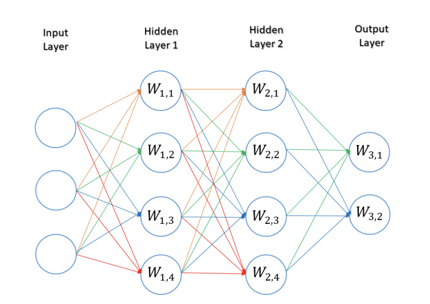
Example of a basic neural network

The neural network in the above example comprises an input layer composed of three input nodes, two hidden layers based on four nodes each, and an output layer consisting of two nodes.

Structure of Feedforward Neural Networks

In a feedforward network, signals can only move in one direction. These networks are considered non-recurrent networks with inputs, outputs, and hidden layers. A layer of processing units receives input data and executes calculations there. Based on a weighted total of its inputs, each processing element performs its computation. The newly derived values are subsequently used as the new input values for the subsequent layer. This process continues until the output has been determined after going through all the layers.

Perceptron (linear and non-linear) and Radial Basis Function networks are examples of feedforward networks. A single-layer perceptron network is the most basic type of neural network. It has a single layer of output nodes, and the inputs are fed directly into the outputs via a set of weights. Each node calculates the total of the products of the weights and the inputs. This neural network structure was one of the first and most basic architectures to be built.

Learning is carried out on a multi-layer feedforward neural network using the back-propagation technique. The properties generated for each training sample are stimulated by the inputs. The hidden layer is simultaneously fed the weighted outputs of the input layer. The weighted output of the hidden layer can be used as input for additional hidden layers, etc. The employment of many hidden layers is arbitrary; often, just one is employed for basic networks.

The units making up the output layer use the weighted outputs of the final hidden layer as inputs to spread the network’s prediction for given samples. Due to their symbolic biological components, the units in the hidden layers and output layer are depicted as neurons or as output units.

Convolutional neural networks (CNNs) are one of the most well-known iterations of the feedforward architecture. They offer a more scalable technique to image classification and object recognition tasks by using concepts from linear algebra, specifically matrix multiplication, to identify patterns within an image.

Below is an example of a CNN architecture that classifies handwritten digits

An Example CNN architecture for a handwritten digit recognition task (source)

Through the use of pertinent filters, a CNN may effectively capture the spatial and temporal dependencies in an image. Because there are fewer factors to consider and the weights can be reused, the architecture provides a better fit to the image dataset. In other words, the network may be trained to better comprehend the level of complexity in the image.

How is a Feedforward Neural Network trained?

The typical algorithm for this type of network is back-propagation. It is a technique for adjusting a neural network’s weights based on the error rate recorded in the previous epoch (i.e., iteration). By properly adjusting the weights, you may lower error rates and improve the model’s reliability by broadening its applicability.

The gradient of the loss function for a single weight is calculated by the neural network’s back propagation algorithm using the chain rule. In contrast to a native direct calculation, it efficiently computes one layer at a time. Although it computes the gradient, it does not specify how the gradient should be applied. It broadens the scope of the delta rule’s computation.

Illustration of the back-propagation algorithm

Structure of Neural Networks

A feedback network, such as a recurrent neural network (RNN), features feedback paths, which allow signals to use loops to travel in both directions. Neuronal connections can be made in any way. Since this kind of network contains loops, it transforms into a non-linear dynamic system that evolves during training continually until it achieves an equilibrium state.

In research, RNNs are the most prominent type of feedback networks. They are an artificial neural network that forms connections between nodes into a directed or undirected graph along a temporal sequence. It can display temporal dynamic behavior as a result of this. RNNs may process input sequences of different lengths by using their internal state, which can represent a form of memory. They can therefore be used for applications like speech recognition or handwriting recognition.

Example of a feedback neural network

How is a Feedback Neural Network trained?

Back-propagation through time or BPTT is a common algorithm for this type of networks. It is a gradient-based method for training specific recurrent neural network types. And, it is considered as an expansion of feedforward networks’ back-propagation with an adaptation for the recurrence present in the feedback networks.

CNN vs RNN

As was already mentioned, CNNs are not built like an RNN. RNNs send results back into the network, whereas CNNs are feedforward neural networks that employ filters and pooling layers.

Application-wise, CNNs are frequently employed to model problems involving spatial data, such as images. When processing temporal, sequential data, like text or image sequences, RNNs perform better.

These differences can be grouped in the table below:

	Convolution Neural Networks (CNNs)	Recurrent Neural Networks (RNNs)
Architecture	Feedforward neural network	Feedback neural network
Layout	Multiple layers of nodes, including convolutional layers	Information flows in different directions, simulating a memory effect
Data type	Image data	Sequence data
Input/Output	The size of the input and output is fixed (i.e, input image with fixed size and outputs the classification)	The size of the input and output may vary (i.e, receiving different texts and generating different translations, for example)
Use cases	Image classification, recognition, medical imagery, image analysis, face detection	Text translation, natural language processing, language translation, sentiment analysis
Drawbacks	Large training data	Slow and complex training procedures
Description	CNN employs neuronal connection patterns. They are inspired by the arrangement of the individual neurons in the animal visual cortex, which allows them to respond to overlapping areas of the visual field.	Time-series information is used by recurrent neural networks. For instance, a user’s previous words could influence the model prediction on what he can says next.

Architecture examples: AlexNet

Alex Krizhevsky developed AlexNet, a significant Convolutional Neural Network (CNN) architecture. This network comprised eight layers: five convolutional layers (some followed by max-pooling) and three fully connected layers. AlexNet notably employed the non-saturating ReLU activation function, which proved more efficient in training compared to tanh and sigmoid. Widely regarded as a pivotal work in computer vision, the publication of AlexNet spurred extensive subsequent research leveraging CNNs and GPUs for accelerated deep learning. By 2022, the AlexNet paper had received over 69,000 citations.

AlexNet Architecture with Pyramid Pooling and Supervision (source)

LeNet

Yann LeCun suggested the convolutional neural network topology known as LeNet. One of the first convolutional neural networks, LeNet-5, aided in the advancement of deep learning. LeNet, a prototype of the first convolutional neural network, possesses the fundamental components of a convolutional neural network, including the convolutional layer, pooling layer, and fully connected layer, providing the groundwork for its future advancement. LeNet-5 is composed of seven layers, as depicted in the figure.

Structure of LeNet-5 (source)

Long short-term memory (LSTM)

LSTM networks are one of the prominent examples of RNNs. These architectures can analyze complete data sequences in addition to single data points. For instance, LSTM can be used to perform tasks like unsegmented handwriting identification, speech recognition, language translation and robot control.

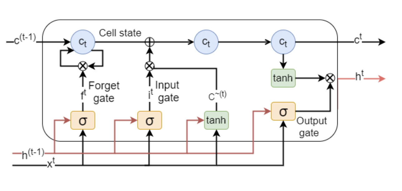
Long Short Term Memory (LSTM) cell (source)

LSTM networks are constructed from cells (see figure above), the fundamental components of an LSTM cell are generally : forget gate, input gate, output gate and a cell state.

Gated recurrent units (GRU)

This RNN derivative is comparable to LSTMs since it attempts to solve the short-term memory issue that characterizes RNN models. The GRU has fewer parameters than an LSTM because it doesn’t have an output gate, but it is similar to an LSTM with a forget gate. It was discovered that GRU and LSTM performed similarly on some music modeling, speech signal modeling, and natural language processing tasks. GRUs have demonstrated superior performance on several smaller, less frequent datasets.

Diagram of the gated recurrent unit cell (Source)

Use cases

Depending on the application, a feedforward structure may work better for some models while a feedback design may perform effectively for others. Here are a few instances where choosing one architecture over another was preferable.

Forecasting currency exchange rates

In a study on modeling the Japanese yen exchange rates, the feedforward model proved to be remarkably straightforward and simple to apply. Despite this simplicity, the model demonstrated strong accuracy in predicting both price levels and price direction for out-of-sample data. Interestingly, the feedforward model outperformed the recurrent network in forecast performance. This could be due to the inherent challenges of models, which often face confusion or instability as they require data to flow both from forward to backward and vice versa.

Recognition of Partially Occluded Objects

There is a widespread perception that feedforward processing is used in object identification. Recurrent top-down connections for occluded stimuli may be able to reconstruct lost information in input images. The Frankfurt Institute for Advanced Studies’ AI researchers looked into this topic. They have demonstrated that for occluded object detection, recurrent neural network architectures exhibit notable performance improvements. Similar findings were reported in the Journal of Cognitive Neuroscience. The experiment and model simulations conducted by the authors emphasize the limitations of the feedforward model in vision tasks. They argue that object recognition is a dynamic and highly interactive process that depends on the collaboration of multiple brain areas, highlighting the complexity beyond simple feedforward processing.

Image classification

In some instances, simple feedforward architectures outperform recurrent networks when combined with appropriate training approaches. For instance, ResMLP, an architecture for image classification that is solely based on multi-layer perceptrons. A research project showed the performance of such a structure when used with data-efficient training. It was demonstrated that a straightforward residual architecture with residual blocks made up of a feedforward network with a single hidden layer and a linear patch interaction layer can perform surprisingly well on ImageNet classification benchmarks if used with a modern training method like the ones introduced for transformer-based architectures.

Text classification

As previously discussed, RNNs are the most successful models for text classification problems. A study proposed three distinct information-sharing strategies to represent text with shared and task-specific layers. All of these tasks are jointly trained over the entire network. The proposed RNN models showed high performance for text classification, according to experiments on four benchmark text classification tasks.

Another paper proposed an LSTM-based sentiment categorization method for text data. This LSTM technique demonstrated sentiment categorization performance with an accuracy rate of 85%, which is considered high for sentiment analysis models.

Conclusion

To put it simply, different tools are required to solve various challenges. It’s crucial to understand and describe the problem you’re trying to tackle when you first begin using machine learning. It takes a lot of practice to become competent enough to construct something on your own; therefore, increasing knowledge in this area will facilitate implementation procedures.

In this post, we looked at the differences between feedforward and feedback neural network topologies. Then we explored two examples of these architectures that have moved the field of AI forward: convolutional neural networks (CNNs) and recurrent neural networks (RNNs). We then gave examples of each structure along with real-world use cases.

Learn more about our products