Decision Tree Regressor
𝐷𝑒𝑐𝑖𝑠𝑖𝑜𝑛 𝑇𝑟𝑒𝑒 𝑐𝑙𝑎𝑠𝑠𝑖𝑓𝑖𝑒𝑟 𝑡ℎ𝑒 𝑚𝑎𝑖𝑛 𝑔𝑜𝑎𝑙 𝑖𝑠 𝑓𝑖𝑛𝑑 𝑡ℎ𝑒 𝑟𝑜𝑜𝑡 𝑛𝑜𝑑𝑒
● 𝐸𝑛𝑡𝑟𝑜𝑝𝑦
● 𝐺𝑖𝑛𝑖
𝐷𝑒𝑐𝑖𝑠𝑖𝑜𝑛 𝑇𝑟𝑒𝑒 𝑟𝑒𝑔𝑟𝑒𝑠𝑠𝑜𝑟 𝑡ℎ𝑒 𝑚𝑎𝑖𝑛 𝑔𝑜𝑎𝑙 𝑖𝑠 𝑓𝑖𝑛𝑑 𝑡ℎ𝑒 𝑟𝑜𝑜𝑡 𝑛𝑜𝑑𝑒
𝐶𝑎𝑙𝑐𝑢𝑙𝑎𝑡𝑒 𝑡ℎ𝑒 𝑀𝑆𝐸 𝑎𝑡 𝑑𝑖𝑓𝑓𝑒𝑟𝑒𝑛𝑡 𝑠𝑝𝑙𝑜𝑡𝑠
𝑥 𝑦
2 10
4 20
6 30
8 40
𝑆𝑡𝑒𝑝 − 1: 𝑠𝑝𝑙𝑖𝑡 𝑡ℎ𝑒 𝑥 𝑎𝑡 𝑑𝑖𝑓𝑓𝑒𝑟𝑒𝑛𝑡 𝑙𝑒𝑣𝑒𝑙𝑠
● 𝑥≥3 𝑜𝑟 𝑥 < 3
● 𝑥≥5 𝑜𝑟 𝑥 < 5
● 𝑥≥6 𝑜𝑟 𝑥 < 6 𝑆𝑡𝑒𝑝 − 2: 𝑙𝑒𝑡𝑠 𝑤𝑜𝑟𝑘 𝑜𝑛 𝑠𝑝𝑙𝑖𝑡 𝑎𝑡 5
● 𝑥≤ 5 𝑛𝑢𝑚𝑏𝑒𝑟 𝑜𝑓 𝑜𝑏𝑠 = 2 𝑖𝑛𝑝𝑢𝑡𝑠 = [2, 4] 𝑜𝑢𝑡𝑝𝑢𝑡(𝑦) = [10, 20]
● 𝑦𝑚𝑒𝑎𝑛 =10+202 = 15
● 𝑚𝑠𝑒1 =(10−15)2+(20−15)22 = 25
● 𝑥 > 5 𝑛𝑢𝑚𝑏𝑒𝑟 𝑜𝑓 𝑜𝑏𝑠 = 2 𝑖𝑛𝑝𝑢𝑡𝑠 = [6, 8] 𝑜𝑢𝑡𝑝𝑢𝑡(𝑦) = [30, 40]
● 𝑦𝑚𝑒𝑎𝑛 =30+402 = 35
● 𝑚𝑠𝑒2 =(30−35)2+(40−35)22
= 25
𝑆𝑡𝑒𝑝 − 3: 𝑇𝑜𝑡𝑎𝑙 𝑚𝑠𝑒 = 𝑤1* 𝑚𝑠𝑒1 + 𝑤2* 𝑚𝑠𝑒2
𝑤1 = 𝑤ℎ𝑒𝑛 𝑥≤5 𝑡𝑤𝑜 𝑖𝑛𝑝𝑢𝑡 𝑜𝑏𝑠𝑒𝑟𝑣𝑎𝑡𝑖𝑜𝑛 𝑎𝑟𝑒 𝑎𝑣𝑎𝑖𝑙𝑎𝑏𝑙𝑒 𝑜𝑢𝑡 𝑜𝑓 𝑡𝑜𝑡𝑎𝑙 (4) =24
𝑤2 = 𝑤ℎ𝑒𝑛 𝑥 > 5 𝑡𝑤𝑜 𝑖𝑛𝑝𝑢𝑡 𝑜𝑏𝑠𝑒𝑟𝑣𝑎𝑡𝑖𝑜𝑛 𝑎𝑟𝑒 𝑎𝑣𝑎𝑖𝑙𝑎𝑏𝑙𝑒 𝑜𝑢𝑡 𝑜𝑓 𝑡𝑜𝑡𝑎𝑙 (4) =24
𝑇𝑜𝑡𝑎𝑙 𝑚𝑠𝑒 =24* 25 +24* 25
𝑟𝑒𝑝𝑒𝑎𝑡 𝑡ℎ𝑒 𝑠𝑎𝑚𝑒 𝑠𝑡𝑒𝑝𝑠 𝑓𝑜𝑟 𝑥 = 3 𝑥 = 7 𝑎𝑛𝑑 𝑠𝑜 𝑜𝑛
𝑐𝑜𝑛𝑐𝑙𝑢𝑠𝑖𝑜𝑛 : 𝑤ℎ𝑖𝑐ℎ 𝑠𝑝𝑙𝑖𝑡 ℎ𝑎𝑠 𝑙𝑜𝑤𝑒𝑠𝑡 𝑀𝑆𝐸 𝑡ℎ𝑎𝑡 𝑏𝑒𝑐𝑜𝑚𝑒 𝑎 𝑏𝑒𝑠𝑡 𝑠𝑝𝑙𝑖𝑡 𝑜𝑛 𝑡ℎ𝑖𝑠 𝑐𝑜𝑙𝑢𝑚𝑛
𝑎𝑠𝑠𝑢𝑚𝑒 𝑡ℎ𝑎𝑡 𝑥 = 5 𝑤𝑒 ℎ𝑎𝑣𝑒 𝑎 𝑙𝑜𝑤 𝑚𝑠𝑒 𝑡ℎ𝑖𝑠 𝑏𝑒𝑐𝑜𝑚𝑒 𝑏𝑒𝑠𝑡 𝑠𝑝𝑙𝑖𝑡 𝑓𝑜𝑟 𝑡ℎ𝑖𝑠 𝑐𝑜𝑙𝑢𝑚𝑛
𝑒𝑥𝑎𝑚𝑝𝑙𝑒 : 𝑠𝑞𝑓𝑡 , 𝑑𝑖𝑠𝑡𝑎𝑛𝑐𝑒, 𝑖𝑛𝑐𝑜𝑚𝑒
𝑐𝑎𝑙𝑐𝑢𝑙𝑎𝑡𝑒 𝑙𝑜𝑤 𝑚𝑠𝑒 𝑎𝑡 𝑒𝑎𝑐ℎ 𝑝𝑜𝑠𝑠𝑖𝑏𝑙𝑒 𝑠𝑝𝑙𝑖𝑡𝑠 𝑓𝑜𝑟 𝑖𝑛𝑐𝑜𝑚𝑒(𝑎𝑠𝑠𝑢𝑚𝑒 50 𝑖𝑛𝑡𝑒𝑟𝑛𝑎𝑙 𝑠𝑝𝑙𝑖𝑡𝑠)
𝑐𝑎𝑙𝑐𝑢𝑙𝑎𝑡𝑒 𝑙𝑜𝑤 𝑚𝑠𝑒 𝑎𝑡 𝑒𝑎𝑐ℎ 𝑝𝑜𝑠𝑠𝑖𝑏𝑙𝑒 𝑠𝑝𝑙𝑖𝑡𝑠 𝑓𝑜𝑟 𝑑𝑖𝑠𝑡𝑎𝑛𝑐𝑒 (𝑎𝑠𝑠𝑢𝑚𝑒 100)
𝑐𝑎𝑙𝑐𝑢𝑙𝑎𝑡𝑒 𝑙𝑜𝑤 𝑚𝑠𝑒 𝑎𝑡 𝑒𝑎𝑐ℎ 𝑝𝑜𝑠𝑠𝑖𝑏𝑙𝑒 𝑠𝑝𝑙𝑖𝑡𝑠 𝑓𝑜𝑟 𝑠𝑞𝑓𝑡(𝑎𝑠𝑠𝑢𝑚𝑒 10 )
𝑜𝑢𝑡 𝑜𝑓 𝑡ℎ𝑒𝑠𝑒 3 𝑤ℎ𝑖𝑐ℎ 𝑖𝑠 𝑎𝑔𝑎𝑖𝑛 𝑙𝑜𝑤𝑒𝑠𝑡 𝑡ℎ𝑎𝑡 𝑏𝑒𝑐𝑜𝑚𝑒 𝑎 𝑟𝑜𝑜𝑡 𝑛𝑜𝑑𝑒
class sklearn.tree.DecisionTreeRegressor(*, criterion=’squared_error’, splitter=’best’, max_depth=None, min_samples_split=2, min_samples_leaf=1, min_weight_fraction_leaf=0.0, max_features=None, random_state=None, max_leaf_nodes=None, min_impurity_decrease=0.0, ccp_alpha=0.0, monotonic_cst=None)[source]
A decision tree regressor.
Read more in the User Guide.Parameters:criterion{“squared_error”, “friedman_mse”, “absolute_error”, “poisson”}, default=”squared_error”
The function to measure the quality of a split. Supported criteria are “squared_error” for the mean squared error, which is equal to variance reduction as feature selection criterion and minimizes the L2 loss using the mean of each terminal node, “friedman_mse”, which uses mean squared error with Friedman’s improvement score for potential splits, “absolute_error” for the mean absolute error, which minimizes the L1 loss using the median of each terminal node, and “poisson” which uses reduction in the half mean Poisson deviance to find splits.
Added in version 0.18: Mean Absolute Error (MAE) criterion.
Added in version 0.24: Poisson deviance criterion.splitter{“best”, “random”}, default=”best”
The strategy used to choose the split at each node. Supported strategies are “best” to choose the best split and “random” to choose the best random split.max_depthint, default=None
The maximum depth of the tree. If None, then nodes are expanded until all leaves are pure or until all leaves contain less than min_samples_split samples.
For an example of how max_depth influences the model, see Decision Tree Regression.min_samples_splitint or float, default=2
The minimum number of samples required to split an internal node:
- If int, then consider
min_samples_splitas the minimum number. - If float, then
min_samples_splitis a fraction andceil(min_samples_split * n_samples)are the minimum number of samples for each split.
Changed in version 0.18: Added float values for fractions.min_samples_leafint or float, default=1
The minimum number of samples required to be at a leaf node. A split point at any depth will only be considered if it leaves at least min_samples_leaf training samples in each of the left and right branches. This may have the effect of smoothing the model, especially in regression.
- If int, then consider
min_samples_leafas the minimum number. - If float, then
min_samples_leafis a fraction andceil(min_samples_leaf * n_samples)are the minimum number of samples for each node.
Changed in version 0.18: Added float values for fractions.min_weight_fraction_leaffloat, default=0.0
The minimum weighted fraction of the sum total of weights (of all the input samples) required to be at a leaf node. Samples have equal weight when sample_weight is not provided.max_featuresint, float or {“sqrt”, “log2”}, default=None
The number of features to consider when looking for the best split:
- If int, then consider
max_featuresfeatures at each split. - If float, then
max_featuresis a fraction andmax(1, int(max_features * n_features_in_))features are considered at each split. - If “sqrt”, then
max_features=sqrt(n_features). - If “log2”, then
max_features=log2(n_features). - If None, then
max_features=n_features.
Note: the search for a split does not stop until at least one valid partition of the node samples is found, even if it requires to effectively inspect more than max_features features.random_stateint, RandomState instance or None, default=None
Controls the randomness of the estimator. The features are always randomly permuted at each split, even if splitter is set to "best". When max_features < n_features, the algorithm will select max_features at random at each split before finding the best split among them. But the best found split may vary across different runs, even if max_features=n_features. That is the case, if the improvement of the criterion is identical for several splits and one split has to be selected at random. To obtain a deterministic behaviour during fitting, random_state has to be fixed to an integer. See Glossary for details.max_leaf_nodesint, default=None
Grow a tree with max_leaf_nodes in best-first fashion. Best nodes are defined as relative reduction in impurity. If None then unlimited number of leaf nodes.min_impurity_decreasefloat, default=0.0
A node will be split if this split induces a decrease of the impurity greater than or equal to this value.
The weighted impurity decrease equation is the following:
N_t / N * (impurity - N_t_R / N_t * right_impurity
                    - N_t_L / N_t * left_impurity)
where N is the total number of samples, N_t is the number of samples at the current node, N_t_L is the number of samples in the left child, and N_t_R is the number of samples in the right child.
N, N_t, N_t_R and N_t_L all refer to the weighted sum, if sample_weight is passed.
Added in version 0.19.ccp_alphanon-negative float, default=0.0
Complexity parameter used for Minimal Cost-Complexity Pruning. The subtree with the largest cost complexity that is smaller than ccp_alpha will be chosen. By default, no pruning is performed. See Minimal Cost-Complexity Pruning for details. See Post pruning decision trees with cost complexity pruning for an example of such pruning.
Added in version 0.22.monotonic_cstarray-like of int of shape (n_features), default=NoneIndicates the monotonicity constraint to enforce on each feature.
- 1: monotonic increase
- 0: no constraint
- -1: monotonic decrease
If monotonic_cst is None, no constraints are applied.Monotonicity constraints are not supported for:
- multioutput regressions (i.e. when
n_outputs_ > 1), - regressions trained on data with missing values.
Read more in the User Guide.
Added in version 1.4.Attributes:feature_importances_ndarray of shape (n_features,)
Return the feature importances.max_features_int
The inferred value of max_features.n_features_in_int
Number of features seen during fit.
Added in version 0.24.feature_names_in_ndarray of shape (n_features_in_,)
Names of features seen during fit. Defined only when X has feature names that are all strings.
Added in version 1.0.n_outputs_int
The number of outputs when fit is performed.tree_Tree instance
The underlying Tree object. Please refer to help(sklearn.tree._tree.Tree) for attributes of Tree object and Understanding the decision tree structure for basic usage of these attributes.
Decision Trees are everywhere in machine learning, beloved for their intuitive output. Who doesn’t love a simple “if-then” flowchart? Despite their popularity, it’s surprising how challenging it is to find a clear, step-by-step explanation of how Decision Trees work. (I’m actually embarrassed by how long it took me to actually understand how the algorithm works.)
So, in this breakdown, I’ll be focusing on the essentials of tree construction. We’ll unpack exactly what’s happening in each node and why, from root to final leaves (with visuals of course).

Definition
A Decision Tree classifier creates an upside-down tree to make predictions, starting at the top with a question about an important feature in your data, then branches out based on the answers. As you follow these branches down, each stop asks another question, narrowing down the possibilities. This question-and-answer game continues until you reach the bottom – a leaf node – where you get your final prediction or classification.

Dataset Used
Throughout this article, we’ll use this artificial golf dataset (inspired by [1]) as an example. This dataset predicts whether a person will play golf based on weather conditions.

Import libraries
from sklearn.model_selection import train_test_split
from sklearn.metrics import accuracy_score
import pandas as pd
import numpy as np
Load data
dataset_dict = {
‘Outlook’: [‘sunny’, ‘sunny’, ‘overcast’, ‘rainy’, ‘rainy’, ‘rainy’, ‘overcast’, ‘sunny’, ‘sunny’, ‘rainy’, ‘sunny’, ‘overcast’, ‘overcast’, ‘rainy’, ‘sunny’, ‘overcast’, ‘rainy’, ‘sunny’, ‘sunny’, ‘rainy’, ‘overcast’, ‘rainy’, ‘sunny’, ‘overcast’, ‘sunny’, ‘overcast’, ‘rainy’, ‘overcast’],
‘Temperature’: [85.0, 80.0, 83.0, 70.0, 68.0, 65.0, 64.0, 72.0, 69.0, 75.0, 75.0, 72.0, 81.0, 71.0, 81.0, 74.0, 76.0, 78.0, 82.0, 67.0, 85.0, 73.0, 88.0, 77.0, 79.0, 80.0, 66.0, 84.0],
‘Humidity’: [85.0, 90.0, 78.0, 96.0, 80.0, 70.0, 65.0, 95.0, 70.0, 80.0, 70.0, 90.0, 75.0, 80.0, 88.0, 92.0, 85.0, 75.0, 92.0, 90.0, 85.0, 88.0, 65.0, 70.0, 60.0, 95.0, 70.0, 78.0],
‘Wind’: [False, True, False, False, False, True, True, False, False, False, True, True, False, True, True, False, False, True, False, True, True, False, True, False, False, True, False, False],
‘Play’: [‘No’, ‘No’, ‘Yes’, ‘Yes’, ‘Yes’, ‘No’, ‘Yes’, ‘No’, ‘Yes’, ‘Yes’, ‘Yes’, ‘Yes’, ‘Yes’, ‘No’, ‘No’, ‘Yes’, ‘Yes’, ‘No’, ‘No’, ‘No’, ‘Yes’, ‘Yes’, ‘Yes’, ‘Yes’, ‘Yes’, ‘Yes’, ‘No’, ‘Yes’]
}
df = pd.DataFrame(dataset_dict)
Preprocess data
df = pd.get_dummies(df, columns=[‘Outlook’], prefix=”, prefix_sep=”, dtype=int)
df[‘Wind’] = df[‘Wind’].astype(int)
df[‘Play’] = (df[‘Play’] == ‘Yes’).astype(int)
Reorder the columns
df = df[[‘sunny’, ‘overcast’, ‘rainy’, ‘Temperature’, ‘Humidity’, ‘Wind’, ‘Play’]]
Prepare features and target
X, y = df.drop(columns=’Play’), df[‘Play’]
Split data
X_train, X_test, y_train, y_test = train_test_split(X, y, train_size=0.5, shuffle=False)
Display results
print(pd.concat([X_train, y_train], axis=1), ‘n’)
print(pd.concat([X_test, y_test], axis=1))
Main Mechanism
The Decision Tree classifier operates by recursively splitting the data based on the most informative features. Here’s how it works:
- Start with the entire dataset at the root node.
- Select the best feature to split the data (based on measures like Gini impurity).
- Create child nodes for each possible value of the selected feature.
- Repeat steps 2–3 for each child node until a stopping criterion is met (e.g., maximum depth reached, minimum samples per leaf, or pure leaf nodes).
- Assign the majority class to each leaf node.

Training Steps
In scikit-learn, the decision tree algorithm is called CART (Classification and Regression Trees). It builds binary trees and typically follows these steps:
- Start with all training samples in the root node.

2.For each feature: a. Sort the feature values. b. Consider all possible thresholds between adjacent values as potential split points.

def potential_split_points(attr_name, attr_values):
sorted_attr = np.sort(attr_values)
unique_values = np.unique(sorted_attr)
split_points = [(unique_values[i] + unique_values[i+1]) / 2 for i in range(len(unique_values) – 1)]
return {attr_name: split_points}
Calculate and display potential split points for all columns
for column in X_train.columns:
splits = potential_split_points(column, X_train[column])
for attr, points in splits.items():
print(f”{attr:11}: {points}”)
- Create two child nodes based on the chosen feature and split point:
- Left child: samples with feature value <= split point
- Right child: samples with feature value > split point

- Recursively repeat steps 2–5 for each child node. You can also stop until a stopping criterion is met (e.g., maximum depth reached, minimum number of samples per leaf node, or minimum impurity decrease).


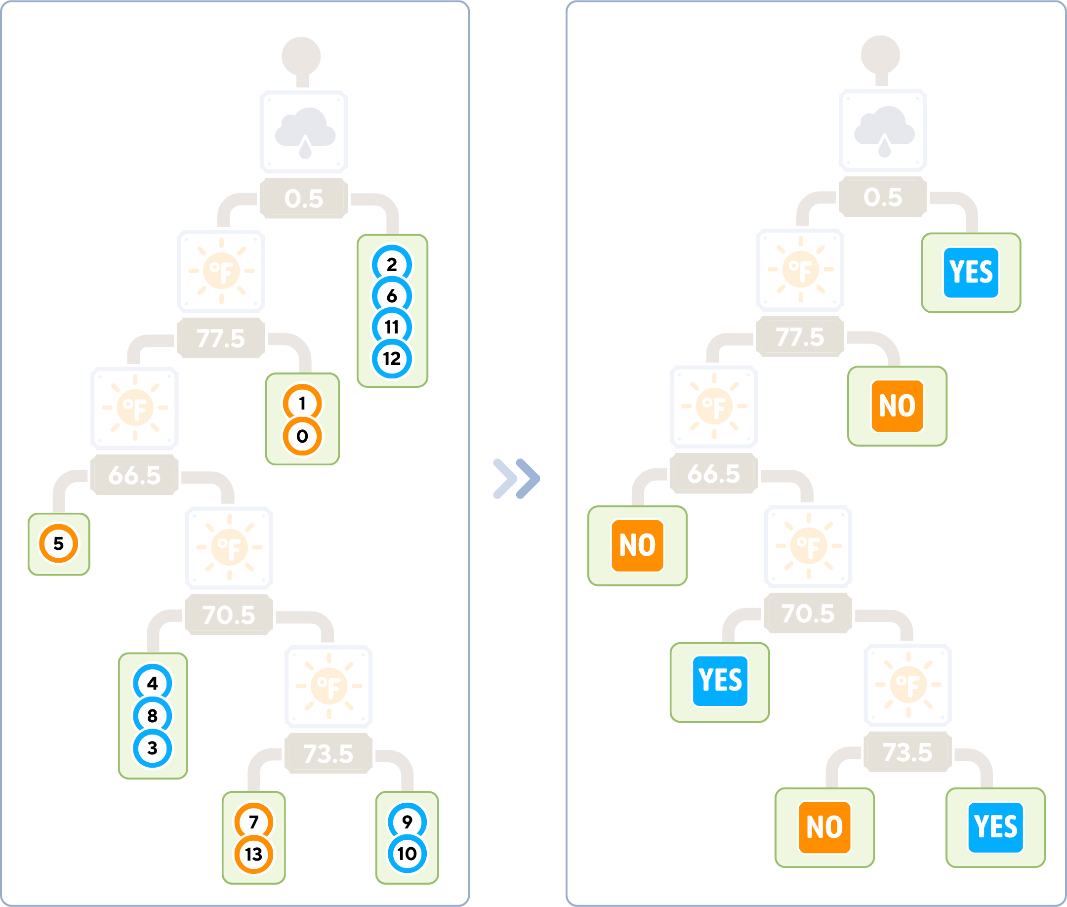
Final Complete Tree
The class label of a leaf node is the majority class of the training samples that reached that node.

# Evaluate the classifier
print(f"Accuracy: {accuracy_score(y_test, y_pred)}")
Key Parameters
Decision Trees have several important parameters that control their growth and complexity:
1 . Max Depth: This sets the maximum depth of the tree, which can be a valuable tool in preventing overfitting.
Helpful Tip: Consider starting with a shallow tree (perhaps 3–5 levels deep) and gradually increasing the depth.

- Min Samples Split: This parameter determines the minimum number of samples needed to split an internal node.
Helpful Tip: Setting this to a higher value (around 5–10% of your training data) can help prevent the tree from creating too many small, specific splits that might not generalize well to new data.

- Min Samples Leaf: This specifies the minimum number of samples required at a leaf node.
Helpful Tip: Choose a value that ensures each leaf represents a meaningful subset of your data (approximately 1–5% of your training data). This can help avoid overly specific predictions.
Pros & Cons
Like any algorithm in machine learning, Decision Trees have their strengths and limitations.
Pros:
- Interpretability: Easy to understand and visualize the decision-making process.
- No Feature Scaling: Can handle both numerical and categorical data without normalization.
- Handles Non-linear Relationships: Can capture complex patterns in the data.
- Feature Importance: Provides a clear indication of which features are most important for prediction.
Cons:
- Overfitting: Prone to creating overly complex trees that don’t generalize well, especially with small datasets.
- Instability: Small changes in the data can result in a completely different tree being generated.
- Biased with Imbalanced Datasets: Can be biased towards dominant classes.
- Inability to Extrapolate: Cannot make predictions beyond the range of the training data.
In our golf example, a Decision Tree might create very accurate and interpretable rules for deciding whether to play golf based on weather conditions. However, it might overfit to specific combinations of conditions if not properly pruned or if the dataset is small.
Final Remarks
Decision Tree Classifiers are a great tool for solving many types of problems in machine learning. They’re easy to understand, can handle complex data, and show us how they make decisions. This makes them useful in many areas, from business to medicine. While Decision Trees are powerful and interpretable, they’re often used as building blocks for more advanced ensemble methods like Random Forests or Gradient Boosting Machines.
Load data
dataset_dict = {
‘Outlook’: [‘sunny’, ‘sunny’, ‘overcast’, ‘rainy’, ‘rainy’, ‘rainy’, ‘overcast’, ‘sunny’, ‘sunny’, ‘rainy’, ‘sunny’, ‘overcast’, ‘overcast’, ‘rainy’, ‘sunny’, ‘overcast’, ‘rainy’, ‘sunny’, ‘sunny’, ‘rainy’, ‘overcast’, ‘rainy’, ‘sunny’, ‘overcast’, ‘sunny’, ‘overcast’, ‘rainy’, ‘overcast’],
‘Temperature’: [85.0, 80.0, 83.0, 70.0, 68.0, 65.0, 64.0, 72.0, 69.0, 75.0, 75.0, 72.0, 81.0, 71.0, 81.0, 74.0, 76.0, 78.0, 82.0, 67.0, 85.0, 73.0, 88.0, 77.0, 79.0, 80.0, 66.0, 84.0],
‘Humidity’: [85.0, 90.0, 78.0, 96.0, 80.0, 70.0, 65.0, 95.0, 70.0, 80.0, 70.0, 90.0, 75.0, 80.0, 88.0, 92.0, 85.0, 75.0, 92.0, 90.0, 85.0, 88.0, 65.0, 70.0, 60.0, 95.0, 70.0, 78.0],
‘Wind’: [False, True, False, False, False, True, True, False, False, False, True, True, False, True, True, False, False, True, False, True, True, False, True, False, False, True, False, False],
‘Play’: [‘No’, ‘No’, ‘Yes’, ‘Yes’, ‘Yes’, ‘No’, ‘Yes’, ‘No’, ‘Yes’, ‘Yes’, ‘Yes’, ‘Yes’, ‘Yes’, ‘No’, ‘No’, ‘Yes’, ‘Yes’, ‘No’, ‘No’, ‘No’, ‘Yes’, ‘Yes’, ‘Yes’, ‘Yes’, ‘Yes’, ‘Yes’, ‘No’, ‘Yes’]
}
df = pd.DataFrame(dataset_dict)
Prepare data
df = pd.get_dummies(df, columns=[‘Outlook’], prefix=”, prefix_sep=”, dtype=int)
df[‘Wind’] = df[‘Wind’].astype(int)
df[‘Play’] = (df[‘Play’] == ‘Yes’).astype(int)
Split data
X, y = df.drop(columns=’Play’), df[‘Play’]
X_train, X_test, y_train, y_test = train_test_split(X, y, train_size=0.5, shuffle=False)
Train model
dt_clf = DecisionTreeClassifier(
max_depth=None, # Maximum depth of the tree
min_samples_split=2, # Minimum number of samples required to split an internal node
min_samples_leaf=1, # Minimum number of samples required to be at a leaf node
criterion=’gini’ # Function to measure the quality of a split
)
dt_clf.fit(X_train, y_train)
Make predictions
y_pred = dt_clf.predict(X_test)
Evaluate model
print(f”Accuracy: {accuracy_score(y_test, y_pred)}”)
Visualize tree
plt.figure(figsize=(20, 10))
plot_tree(dt_clf, filled=True, feature_names=X.columns,
class_names=[‘Not Play’, ‘Play’], impurity=False)
plt.show()