A warmer atmosphere holds more water. Scientists have spent decades using that fact as a foundation: wet tropical regions would get wetter, dry ones drier, with rain deepening in place as the planet heats. The models all pointed the same direction.
The tropics have pointed somewhere else. Over more than four decades the belts of equatorial downpour have crept northward in ways those models did not anticipate, and a new study traces the cause to dry land. The expectation even had a clear name. For years scientists leaned on the wet-get-wetter rule, the notion that warming would bring more rain to already-soggy regions and pull it from dry ones. Tropical rainfall was supposed to follow. Changing the world starts with how we see it
At the University of Southampton, we believe progress starts with people willing to think differently – who have the curiosity to explore, the confidence to question and the ambition to create momentum.

They lined up weather and satellite records from 1979 to 2024 against the models meant to reproduce them.
Nothing lined up. Rain across the tropics had moved and regrouped along lines standard physics could not explain alone, sending the team hunting for a different driver.
Rain on the move
The clearest signal sat over the Pacific. More rain was falling north of the equator, over the western Pacific, the islands of Southeast Asia, and India, while a band just south and much of South America dried out. Human-caused Indo-Pacific warm pool expansion. The Indo-Pacific warm pool (IPWP) has warmed and grown substantially during the past century. The IPWP is Earth’s largest region of warm sea surface temperatures (SSTs), has the highest rainfall, and is fundamental to global atmospheric circulation and hydrological cycle. The region has also experienced the world’s highest rates of sea-level rise in recent decades, indicating large increases in ocean heat content and leading to substantial impacts on small island states in the region. Previous studies have considered mechanisms for the basin-scale ocean warming, but not the causes of the observed IPWP expansion, where expansion in the Indian Ocean has far exceeded that in the Pacific Ocean. We identify human and natural contributions to the observed IPWP changes since the 1950s by comparing observations with climate model simulations using an optimal fingerprinting technique. Greenhouse gas forcing is found to be the dominant cause of the observed increases in IPWP intensity and size, whereas natural fluctuations associated with the Pacific Decadal Oscillation have played a smaller yet significant role. Further, we show that the shape and impact of human-induced IPWP growth could be asymmetric between the Indian and Pacific basins, the causes of which remain uncertain. Human-induced changes in the IPWP have important implications for understanding and projecting related changes in monsoonal rainfall, and frequency or intensity of tropical storms, which have profound socioeconomic consequences. Tropical rain belts and great monsoons are creeping northward, defying traditional climate models that predicted a uniform deepening of rain over existing wet zones. Driven by rapid warming over northern landmasses and a massive expansion of the warm ocean pool around Indonesia, these shifts are throwing seasonal rainfall patterns out of sync. Consequently, the agricultural lifelines of India, West Africa, and Southeast Asia face severe disruption. The expectation even had a clear name. For years scientists leaned on the wet-get-wetter rule, the notion that warming would bring more rain to already-soggy regions and pull it from dry ones. Tropical rainfall was supposed to follow.The Indo-Pacific warm pool (IPWP), where sea surface temperatures (SSTs) exceed 28°C (which is an estimated threshold for atmospheric deep convection), supports the Walker circulation’s rising branch and largely determines rainfall distribution throughout the tropics to extratropics. It plays a key role in climate and monsoon variability for many developing countries throughout Asia and Africa, but also influences remote regions and large-scale climate modes of variability. From year to year, IPWP intensity and size fluctuate with the El Niño–Southern Oscillation (ENSO). The ongoing IPWP warming and expansion in recent decades are, by one estimate, responsible for more tropical Indo-Pacific SST variance than anomalies associated with ENSO .
Recent studies suggest greenhouse gas–induced warming to be the major cause for global ocean temperature and tropical Indian Ocean SST changes, but its role in the observed IPWP region changes is not clear. We provide the first quantitative attribution of the observed IPWP warming and expansion changes during the past 60 years, examining anthropogenic and natural contributions to the IPWP warming and expansion. We address this by comparing observed 1953–2012 changes with climate model–simulated changes using CMIP5 (Coupled Model Intercomparison Project Phase 5) historical climate change simulations that account for anthropogenic forcing (greenhouse gases, aerosols, and other anthropogenic forcing agents) combined with natural (solar and volcanic activities) forcings (ALL), greenhouse gas forcing only (GHG), or natural forcings only (NAT).
RESULTS
Observed and modeled changes
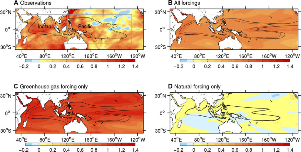
Models simulate the observed Indo-Pacific warming and IPWP expansion reasonably well, albeit with greater warming and expansion in the central to eastern Pacific (fig. S1), a region affected by persistent biases (for example, excessively strong equatorial Pacific cold tongue). We focus our analysis on 29 of 42 models (tables S1 and S2; see Materials and Methods) that simulate a realistic IPWP (that is, comparable size to observations; fig. S2) to reduce the impact of biases because there is a close relationship between IPWP mean size with changes in intensity and area (fig. S3). Specific forcing experiments show that realistic changes occur only when greenhouse gases are included (Fig. 1B to D) but that the response is stronger than observed in GHG-only experiments, which exclude negative contributions from other anthropogenic forcings, such as aerosols.
To examine long-term IPWP intensity and area changes, we considered non overlapping 5-year annual means over the 60-year period. Mean IPWP SST and area are calculated over the Indo-Pacific region enclosed by the 28°C isotherm between 25°S to 25°N and 40°E to 130°W. We also independently analyze the Indian and Pacific Ocean warm pools. The IPWP warmed and expanded steadily until the late 1990s, followed by weaker trends, as observed in global mean temperature. The ALL and anthropogenic forcing (ANT; estimated as ALL minus NAT) simulations show realistic increasing trends, whereas GHG-only trends are significantly larger than observed. In contrast, NAT-only simulations have varying decadal trends, resulting in no significant long-term trend. The signal induced by ANT-only is therefore close to that from ALL forcing. Preindustrial control simulations from the models are used to provide a measure of the range of trends arising from unforced internal climate variability, which the observed trends exceed.
| SALL (SNRALL) | SANT (SNRANT) | SGHG | SNAT | NCTL | SOBS SOBS* | |
|---|---|---|---|---|---|---|
| Intensity (°C per 60 years) | ||||||
| Indo-Pacific | 0.25 (7.24) | 0.24 (7.01) | 0.39 | 0.01 | 0.03 | 0.30 (0.26*) |
| Indian | 0.26 (9.16) | 0.25 (8.97) | 0.43 | 0.01 | 0.03 | 0.34 (0.28*) |
| Pacific | 0.28 (6.14) | 0.27 (6.02) | 0.43 | 0.01 | 0.05 | 0.33 (0.29*) |
Table 1 Comparison of trends in warm pool intensity and area between observations and climate model simulations.
Multimodel means of linear trend slopes are defined as the signal (SALL, SANT, SGHG, or SNAT), and the SD of trends across nonoverlapping CTL chunks is defined as the noise (N). Signal-to-noise ratios (SNRs) are then calculated from slopes of SST and area series averaged over the three warm pool regions during 1953–2012 for ALL and ANT simulations. Observational trend slopes with (SOBS) and without the influence of the PDO (SOBS*) are given for comparison. Units for S and N are °C and % per 60 years for warm pool intensity and area, respectively.
Despite studies reporting tropical Indian Ocean warming at a rate of up to three times faster than the tropical Pacific (fig. S4A), trends are comparable if only area-mean SSTs averaged in the expanding warm pool of both oceans are compared, due to the larger increase in warm pool size in the Indian Ocean. Therefore, the zonal intensity gradient (Indian minus Pacific) between the two warm pool sectors has experienced little change (fig. S4B). Year-to-year variations of approximately 10 to 15% (relative to the climatological mean) in IPWP size occur with ENSO, far less than the observed expansion of over 30% since the 1950s. Warm pool expansion in the Indian Ocean (51%) has also far exceeded that in the Pacific Ocean (22%). These results are consistent among observational data sets despite some regional differences, and are different to similar expansion rates in both basins associated with a uniform warming (fig. S5).
Detection of human influence
To detect and quantify contributions from ALL, GHG, ANT, and NAT forcings to long-term variations in IPWP intensity and area, we use an optimal fingerprinting technique. In this method, observations are regressed via generalized linear regression onto one or two multimodel-simulated signals (see Materials and Methods for details). We conduct single-signal analyses by regressing observations onto model-simulated responses to ALL, ANT, GHG, and NAT forcings estimated from the average of the selected model ensemble. We conduct a two-signal analysis in which observations are simultaneously regressed onto ANT and NAT response to estimate the contribution of both anthropogenic and natural forcings to changes in warm pool properties. Unforced control (CTL) simulations are used to obtain an estimate of the internal climate variability, in addition to conducting a residual consistency test to compare model-simulated internal variability with observations. Resulting best estimates and uncertainty ranges of scaling factors, which scale estimates of the responses to individual combinations of forcings to best reproduce observed changes, are used to determine whether external forcings are present in observations. Intensity and area changes are not perfectly correlated (r = 0.87, P < 0.01), and thus, we combine normalized intensity and area anomalies to capture additional information on changes that may improve detection and attribution. The influence of external forcing is detected when a scaling factor is significantly greater than zero, and considered consistent with observations when it is consistent with unity.
Scaling factors based on single-signal optimal analyses are shown in the left panels. Except for the Pacific warm pool area, scaling factors for ALL, GHG, and ANT are significantly greater than zero for long-term warm pool intensity and area changes, including combined changes. This indicates that the overall effect of external anthropogenic and natural forcing, or the effect of greenhouse gas forcing or anthropogenic forcing alone, can be detected. In most cases, uncertainty ranges for the scaling factors on the ALL and ANT responses include unity, indicating consistency with observations. Best estimates for ALL and ANT scaling factors are slightly above one for warm pool intensities and Indian Ocean warm pool area (Fig. 3,A and B), highlighting some underestimation of the response in the multimodel mean. In contrast, best estimates for GHG are below one, meaning that GHGs acting alone would have produced larger changes than the observed. Strong agreement of best estimates with observed trends is found in all three warm pool regions when combining intensity and area changes. The influence of NAT is not robustly detected in any case considered. The residual consistency test is passed in most of the single-signal cases, indicating that the residual variability that remains in the observations after removing the scaled response is consistent with model internal variability.
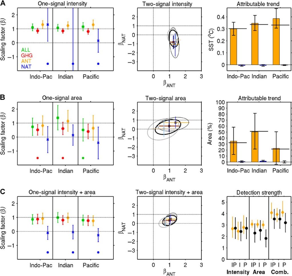
Results from two-signal (ANT and NAT) analyses of warm pool intensity and area changes are shown in the center panels. The ANT influence is detected in all cases with clear separation from the NAT influence except for the Pacific warm pool area. The ANT scaling factors for IPWP changes are closest to unity with more confidence compared to the Indian and Pacific Oceans separately. Overall, ANT signals for warm pool intensity must be scaled up, and ANT signals for warm pool area need to be scaled up for the Indian Ocean, but CIs encompass unity. NAT is not robustly detected because the joint confidence ellipses include zero on the NAT axis in all cases.
ANT-attributable trends (calculated by multiplying two-signal scaling factors with multimodel mean trends) are very close to observed intensity and area trends. Considering combined changes increases the “detection strength,” which is a representation of the projection of any model run or observations onto the single variable or combined fingerprint, and further increases confidence that intensity and area changes are not due to internal variability alone . Our detection results are robust to the use of different SST data sets and different model sampling (see Materials and Methods).
Internal variability influence
To understand the models’ underestimation of the warm pool warming, we assess the contribution of internal climate variability evident in observations. The dominant mode of multidecadal variability in the Indo-Pacific is the Pacific Decadal Oscillation (PDO). Changes in IPWP intensity and area associated with the observed PDO variability during the last 60 years have augmented that due to anthropogenic forcing. The contribution of the PDO to the observed IPWP warming and expansion is approximately 12 to 18%. Removing the PDO influence from observations (based on linear regression) results in better agreement with multimodel anthropogenic responses in intensity trends and Indian Ocean warm pool expansion.
Impact of IPWP changes
We investigate the impact of the nonuniform IPWP changes focusing on rainfall responses using observations and CMIP5 models. On the basis of the observations for the satellite period, different rainfall change patterns appear to be more associated with individual Indian and Pacific warm pool changes than for the IPWP as a whole (fig. S6). This emphasizes the importance of the regional IPWP warming patterns in terms of IPWP’s impacts and teleconnections. Satellite period observations show more warming and larger expansion in the Indian Ocean warm pool than in the Pacific, together with an intensification and westward shift in precipitation change, even after accounting for the influence of internal variability during this period (fig. S7, A and B). The notion that the asymmetric response in the IPWP changes is not due to fluctuations of internal variability is supported by the CMIP5 models because they exhibit no relationship between the ratio of Indian and Pacific warm pool expansion with the PDO trend over a 60-year period (fig. S7C). We use CMIP5 models to further explore the individual impacts of Indian and Pacific Ocean warm pool warming and expansion on rainfall. To do so, we have selected two groups of models: one with trends in IPWP intensity and area similar to those observed, that is, with stronger warming and expansion trends in the Indian Ocean than in the Pacific Ocean (five models; refer to caption in fig. S8), and another group with opposite trends (six models). Note that we use a longer period of 1953–2012 to focus on long-term responses, different from the observed period (1979–2012).
Regional precipitation patterns are determined by relative changes in the spatial pattern of the tropical SST climatology. Given the large intermodel differences in tropical SST climatology and trends, one cannot expect good intermodel agreement in rainfall responses. Accordingly, our results show generally low agreement in rainfall trends except in a few regions (fig. S8). In particular, models with larger expansion in the Indian Ocean, like the recent observations, tend to have increased rainfall over the western Indian Ocean that resembles the observed trend. In contrast, models with stronger warm pool warming and expansion in the western Pacific exhibit a decrease in precipitation over Southeast Asia. This model-simulated drying response is consistent with previous findings, which describe the major role of zonal SST difference between the tropical Indian Ocean and western Pacific Ocean in determining the strength of the western Pacific subtropical high and thus affecting East Asian monsoon rainfall and western Pacific tropical cyclone activity. Australian rainfall response in models is also consistent with recent finding, which indicate that a warming Indian Ocean warm pool induces rainfall increase, whereas a warming Pacific warm pool leads to rainfall reduction (fig. S8). The spatial pattern of difference in rainfall trends between the two model groups (models with larger expansion in the Indian Ocean minus models with larger expansion in the Pacific Ocean) is very similar to the observed pattern of trends (compare fig. S8C with fig. S7), confirming the importance of the area of SST contrast between the two warm pool areas. The individual models help highlight the large spread that still exists in models with similar changes in expansion of the IPWP, explaining why we see only limited regions of significant change (fig. S8D). For example, the difference in the western Indian Ocean is significant (at the 1% level) between the two model groups because the realistic models all simulate the increase in rainfall. Conversely, the opposite is seen for the East Asian region, where models that simulate larger Pacific expansion have a decrease in rainfall, again consistent with previous modeling studies, which showed that a significant drying response over East Asia is primarily associated with stronger Pacific warming. Consistent with the observations, the ensemble mean of models with the more realistic larger Indian Ocean expansion does not simulate an increase in the East Asia region. In the observations, the small significant region of drying over East Asia is removed once the PDO is accounted for (fig. S7). This corroborates previous findings that the negative PDO-like SST pattern that prevailed during the recent hiatus period explains pronounced regional drying anomalies in this region.
Regions of deep convection are integral to the large-scale circulation in the tropics and closely tied to areas of warm SSTs. However, the size of this region of convection has been shown to remain relatively constant in a warming world, suggesting that the convective threshold increases with SST and that precipitation intensity increases within the region that lies above the changing convective threshold. We have therefore also examined convection changes that correspond to IPWP changes based on a simple analysis of CMIP5 models. We find that rainfall intensity modestly increases with warming in the IPWP in most of the models, but the convection area (diagnosed as the area with precipitation > 2 mm day−1) changes very little (fig. S9). In contrast to the warm pool expansion, both basins experience a similar increase in warm pool intensity, and thus, simulated changes in precipitation increase as described in previous studies and as observed. Overall, although the convection area does not vary significantly in the long term as the convection threshold increases with SST, covering about 25% of the global ocean, its location has undergone a significant shift westward with a relatively larger area with SSTs above the convection threshold in the Indian Ocean.
DISCUSSION
Our results identify contributions from anthropogenic forcings (mainly greenhouse gas increase) and natural causes (the PDO) to observed IPWP warming and expansion during the last 60 years. This quantitative attribution of the influence of anthropogenic forcing and also assessment of climate variability increases confidence in the understanding of the causes of past changes as well as for projections of future changes under further greenhouse warming. Expansion of the IPWP due to anthropogenic forcing will likely continue; however, shifts in the mean state of the tropical ocean could change the relative amounts of expansion in the two adjacent oceans and modulate the long-term change in the IPWP impact. This has important implications for many vulnerable regions. For example, stronger than normal summer Indian monsoons are preceded by an expanding and warming Indian Ocean warm pool. A mean state change in this direction could also affect East Asian climate by inducing a westward extension of the western Pacific subtropical high. In addition to long-term trends, decadal variability in IPWP intensity and size can directly affect the Hadley and Walker circulations, inducing corresponding changes in rainfall even in the extratropics. This means that understanding and predicting changes of the IPWP mean state as well as regional contrast is critical to reliable future projections of changes in global and regional atmospheric circulation and hydrological cycle.
MATERIALS AND METHODS
Data processing
We used SST from HadISST (Hadley Centre sea ice and SST) v1.1 and ERSST (Extended Reconstructed SST) v3b data sets for the period 1953–2012 to calculate properties of the IPWP (for example, intensity and area). The area enclosed by the 28°C isotherm for the Indo-Pacific sector between 25°S to 25°N and 40°E to 130°W was obtained using the monthly data. The mean seasonal cycle of intensity and area calculated for 1953–2012 was removed to obtain monthly anomaly information. Annual mean anomalies were constructed for analysis and comparison with model simulations. We assessed the relationship between warm pool properties (SST intensity and area greater than 28°C) and rainfall in the satellite era (1979–2012) with GPCP (Global Precipitation Climatology Project) monthly precipitation analysis data.
We used 42 CMIP5 models forced with historical anthropogenic and natural forcings (1953–2005) and future greenhouse gases under emission scenario of Representative Concentration Pathway (RCP) 4.5 (2006–2012), covering a 60-year period (table S1). The climatological size of the IPWP (area bounded by the 28°C isotherm) was used to select a subset of models. Of the 42 models, 29 satisfy the criterion whereby the size of the model’s climatological IPWP lies within the observed average ± 1 SD of the observed interannual variability (fig. S2). The selected models yield a mean IPWP area of 46.0 × 10¹² m2, close to the observed area in HadISST of 43.9 × 10¹² m2 (table S2). In total, 80 simulations of the historical period were used, referred to as the ALL forcing experiment. Individual forcing simulations using greenhouse gases only (GHG-only) and external natural forcing only (NAT-only) were obtained from the selected models (if available), with a total of 25 and 29 simulations, respectively.
All model outputs were regridded to a common 1° × 1° latitude/longitude grid, then ensemble means were first calculated for individual models, and multimodel means were obtained by taking arithmetic averages of the model-specific ensemble means, giving equal weight to each model when constructing multimodel means. We estimated the anthropogenic forced (ANT) signal as the difference between ALL and NAT under the assumption of linearly additive responses to the external forcings. Preindustrial control (CTL) simulations (19,800 years, which provided 333 nonoverlapping 60-year chunks in total) from all available models were used to estimate the characteristics of model unforced internal climate variability to increase number of independent noise data, which helps reduce sampling uncertainty in covariance estimation of the internal climate variability (42). Using CTL simulations from the 29 selected models did not affect main results.
Detection method
To compare observed and modeled warm pool intensity and area anomaly time series, an optimal fingerprinting technique was used. Observations (y) were regressed onto multimodel mean response patterns (X, fingerprints of ALL, ANT, GHG, and NAT) such that y = (X − ν)β + ε. Here, regression coefficients β (or scaling factors) are obtained by the total least squares method, ν represents the component of X due to internal variability that remains after multimodel averaging, and ε represents the residual variability that is generated internally in the climate system. The variance-covariance matrix of ε is estimated from preindustrial control (CTL) simulations, and that of ν is taken to be proportional to the variance-covariance matrix of ε, where the constant of proportionality reflects the methods used to calculate the multimodel ensemble response patterns. We conducted two regression analyses. (i) Single-signal analyses were performed by linearly regressing observations onto single (ALL, ANT, GHG, or NAT) fingerprints to examine whether the signal considered is present in the observed changes. (ii) A two-signal analysis was undertaken whereby observations were regressed onto ANT and NAT simultaneously. This allows an examination of whether ANT and NAT are jointly detected and whether the influence of ANT is separable from that of NAT and internal variability in the observations. We divided 60-year chunks of CTL simulations into two sets (116 chunks each) for the optimal fingerprinting analysis. The first set was used to obtain best estimates of β, and the other set was used to estimate the 5 to 95% uncertainty range for β and also to carry out a standard residual consistency test. This test offers a convenient method to check whether model-simulated internal variance is consistent with observational residual variance. Because the key aspect of this study was on long-term variability of warm pool intensity and area changes, we calculated 5-year mean time series of anomalies to reduce noise on interannual time scales. Therefore, 12-dimensional data vectors of observations and model simulations were obtained. Because data vectors have low dimension compared to the number of chunks of CTL simulations available for covariance matrix estimation (12 dimensions versus 115 chunks for each of the two covariance matrix estimates), we did not apply further dimension reduction, such as empirical orthogonal function truncations.
We assessed the sensitivity of different model samples to forcing signals and optimal fingerprinting analysis by using six models that had ALL, GHG, and NAT simulations. This evaluation also allowed an assessment of the sensitivity of the calculation of the anthropogenic forcing as the difference between ALL and NAT to the use of multimodel means from different samples of models. The results were found to be robust regardless of model samples used (compare with figs. S10 and S11). For example, long-term trends (fig. S10) and scaling factors from optimal fingerprinting results (fig. S11) were found to be robust to the use of different multimodel ensembles. As this warm pool has grown, it has drawn moist air toward the islands and fed the rain spreading north.

Climate change is hitting wildlife hardest in unexpected places where climate change is hitting wildlife hardest, and most people point to the tropics – rainforests, coral reefs, and species adapted to a narrow range of temperatures. For a long time, scientists agreed. A sweeping new look at thousands of plant and animal species suggests that long-held assumption is now backwards.
A surprising reversal

Local species extinctions are often underestimated Biodiversity time series are biased towards increasing species richness in changing environments discrepancy between global loss and local constant species richness has led to debates over data quality, systematic biases in monitoring programmes and the adequacy of species richness to capture changes in biodiversity. We show that, more fundamentally, null expectations of stable richness can be wrong, despite independent yet equal colonization and extinction. We analysed fish and bird time series and found an overall richness increase. This increase reflects a systematic bias towards an earlier detection of colonizations than extinctions. To understand how much this bias influences richness trends, we simulated time series using a neutral model controlling for equilibrium richness and temporal autocorrelation (that is, no trend expected). These simulated time series showed significant changes in richness, highlighting the effect of temporal autocorrelation on the expected baseline for species richness changes. The finite nature of time series, the long persistence of declining populations and the potential strong dispersal limitation probably lead to richness changes when changing conditions promote compositional turnover. Temporal analyses of richness should incorporate this bias by considering appropriate neutral baselines for richness changes. Absence of richness trends over time, as previously reported, can actually reflect a negative deviation from the positive biodiversity trend expected by default. The expectation that species richness remains constant in the absence of external forcing at ecological time scales is deeply rooted in ecological theories assuming a dynamic equilibrium between colonizations and extinctions. Assessments of time series in the global change context thus interpret deviations from balanced dynamics such as positive and negative trends in species number as a response to improving or deteriorating environmental conditions, respectively. Under increased environmental suitability (Fig. 1), most species will profit, and the expected positive trends emerge, although colonizations may also be delayed (‘immigration credit). On the other hand, one can expect that a reduction in habitat suitability will affect most species negatively up to the extinctions of some (Fig. 1). As the exponential decline of existing populations takes time (for example, because of plasticity, use of microrefugia), extinction debts will lead to a delayed reduction in richness and the negative richness trends will only emerge later.
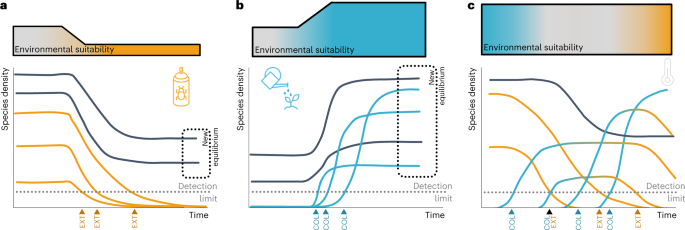
Yellow lines indicate species experiencing population declines up to extinction while blue ones indicate species experiencing increases in density. a, The case of a negative impact (for example, increase in pesticides, habitat fragmentation) resulting in a lower equilibrium richness, which can take some time to establish as declining populations persist (extinction debt). b, A clear positive impact (for example, enlargement of habitat size through restauration) that leads to a higher equilibrium richness, which might take time to establish as gained populations need some time to colonize (immigration credit). c, A steady change: even though as many species decline (that is, ‘losers’) as colonize (that is, ‘winners’), the observed richness increases if new species arrive earlier than species go extinct. This increase does not disappear, as any new time segment added leads again to earlier colonizations than extinctions, with no new equilibrium being reached. EXT, extinction; COL, colonization.
The scale- and effort-dependency of species richness as a metric creates uncertainty around trends, while, in addition, richness does not capture compositional turnover but rather the net difference between colonizations and extinctions. Even more fundamentally though, the temporal response of richness might not match our expectation, especially if the environment-driven trajectory is not clearly negative or positive but neutral, as some species are favoured and can colonize while others decline and eventually go extinct.
To conceptualize the issue, consider a neutral environmental change such that there are equal numbers of ‘winners’ and ‘losers’, and richness is expected to remain constant. However, under low dispersal limitation, one can assume that colonizations (defined as the first colonization event over a given time series) will be fast (as it needs only few propagules), whereas extinctions (defined as the last extinction event over a given time series) will be delayed because in the absence of catastrophic mortality population growth will slowly turn negative for the losers. For dominant species, the resulting decline in abundance will result in extinction after many generations. This extinction process might be further slowed down if density-dependent mortality declines or populations adapt their phenotypes to the new conditions. This bias towards earlier colonizations will result in increasing richness over time, which may be transient if the environmental change stops at some point such that colonizations and extinctions can equilibrate again. However, if environmental change continues, each incremental increase in observation time will allow further colonizations, resulting in further imbalance detected as increasing richness in finite time series. On the other hand, if a community exhibits a strong inertia in its dynamics, rare species are likely to go extinct and not locally recolonize. Thus, as the majority of species are rare, decrease in richness will emerge.
Results and discussion
Temporal trends in species richness
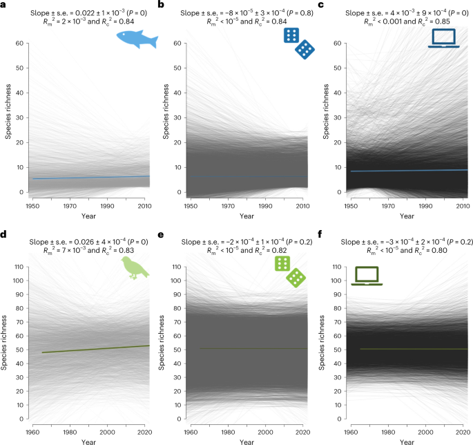
Here, we combine observational data and simulations to test whether this imbalance is strong enough to fundamentally shift species richness trends to slopes different from zero by default. We first analysed species richness trends using 3,036 European empirical freshwater fish community time series from the highly curated RivFishTIME dataset (average duration = 24 years), along with 4,317 time series from the Breeding Bird Survey in North America (average duration = 37 years). Across the empirically sampled communities, the average slopes from the linear mixed-effects (LME) model were +0.02 (standard error (s.e.) = 0.001, P < 0.001, marginal R2 = 0.002, conditional R2 = 0.85) and +0.03 (s.e. = 0.0001, P < 0.001, marginal R2 = 0.007, conditional R2 = 0.83) for freshwater fish and breeding bird communities, respectively. The empirical data thus correspond to previous meta-analyses, showing no overall decline in local richness, but rather a small yet significant average increase over time.
Shorter time series revealed more variable estimates for slopes and larger standard errors (Supplementary and Supplementary Tables). To test whether the positive overall richness trend was driven by short time series only, we used a generalized additive model for location scale and shape (GAMLSS). While only the variance in species richness trends was affected by time series length for freshwater fish (estimateslope ± s.e. = 1 × 10⁻⁵ ± 1 × 10⁻⁵, P = 0.3; estimatevariance ± s.e. = −0.04 ± 2 × 10⁻³, P < 0.001; R2 = 0.20), both the mean and the variance in species richness trends were impacted for birds (estimateslope ± s.e. = 1 × 10⁻⁵ ± 1 × 10⁻⁶, P < 0.001; estimatevariance ± s.e. = −0.03 ± 8 × 10⁻⁴, P < 0.001; R2 = 0.29). Thus, when dispersal is not strongly constraining communities (for example, avian communities), short time series exhibit a duration-related underestimation bias in the observed trends. While we fully acknowledge the time and money already needed to collect such data, we need to accept that most currently used worldwide long-term datasets actually capture relatively short time series. Therefore, our results strongly suggest that short time series potentially underestimate diversity loss, as previously claimed.
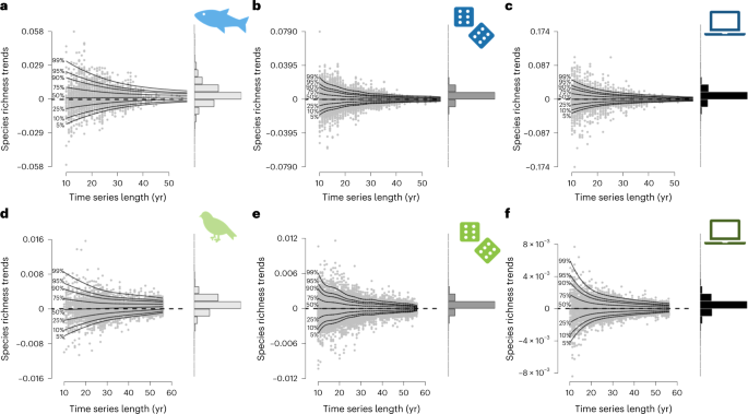
We compared these observations with a null model for which we fully randomized the observed yearly chronosequences of species, thereby fully removing temporal autocorrelation from year to year in species dynamics. Such null models are often used to provide a benchmark for a given diversity metric in the absence of driving processes. For both taxa-specific null models, species richness was steady over time (LME, fish: estimate ± s.e. = −8 × 10⁻⁵ ± 3 × 10⁻⁴, P = 0.8, marginal R2 < 0.001, conditional R2 = 0.84; birds: estimate ± s.e. = −2 × 10⁻⁴ ± 1 × 10⁻⁴, P = 0.2, marginal R2 < 0.001, conditional R2 = 0.82), while the variance was reduced under long time series (fish: estimatevariance ± s.e. = −5 × 10⁻² ± 5 × 10⁻⁴, P < 0.001, R2 = 0.30; birds: estimatevariance ± s.e. = −4 × 10⁻² ± 3 10−4, P < 0.001, R2 = 0.48). However, this classic null model approach is highly unrealistic for biodiversity time series as it allows any species to flip between absence, rare and abundant occurrences, which does not occur in actual populations. In the absence of catastrophic extinctions, the population size at any time point is correlated with the abundance at the previous time step via the specific birth and death rates, resulting in strong temporal autocorrelation under regular monitoring when sampling intervals are not very large compared with generation time.
To analyse whether incorporating temporal autocorrelation matters for null expectations, we simulated 9,999 time series of neutral communities. These simulations matched the empirical observations with respect to mean and variance of time series length and species richness. We derived these time series from a neutral model based on the theory of island biogeography, simulating species occurrences while controlling for equilibrium richness and temporal autocorrelation. We explored a large range of autocorrelations (Supplementary Table 1), but highlight a case with an autocorrelation level matching the observed temporal autocorrelation. Despite being a neutral model, simulated time series for river fish exhibited increased species richness over time (estimate ± s.e. = 4 × 10⁻³ ± 9 × 10⁻⁴, P < 0.001, marginal R2 < 0.001, conditional R2 = 0.85), which suggests that these fish communities are not at equilibrium with their historical context. By contrast, simulated time series for breeding birds did not show a significant deviance from neutral trends (estimate ± s.e. = −3 × 10⁻⁴ ± 2 × 10⁻⁴, P = 0.2, marginal R2 < 0.001, conditional R2 = 0.80), which may reflect that bird communities are less constrained in their dispersal, allowing stronger rescue effect. The simulated slope of richness over time was significantly independent from time series length (fish: estimateslope ± s.e. = −6 × 10⁻⁶ ± 1 × 10⁻⁵, P = 0.6, R2 = 0.20; birds: estimateslope ± s.e. = 2 × 10⁻⁷ ± 4 × 10⁻⁷, P = 0.7, R2 = 0.48), only variance in species richness trends decreased with longer time series (fish: estimatevariance ± s.e. = −5 × 10⁻² ± 9 × 10⁻⁴, P < 0.001; birds: estimatevariance ± s.e. = −4 × 10⁻² ± 5 × 10⁻⁴, P < 0.001). This pattern holds for most of the settings of autocorrelation and balance between colonization and extinction we have tested . Thus, the observed departure from a zero slope for simulated data, especially in the case of riverine fish, is not linked to the empirical time series being too short.
Net imbalance between colonizations and extinctions
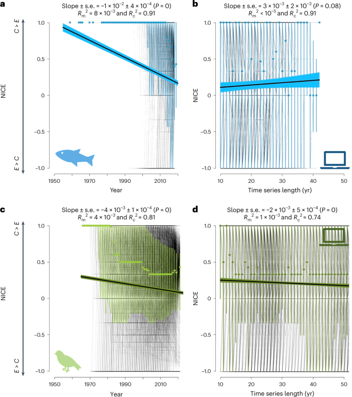
Richness increases are inevitable when population dynamics exhibit strong autocorrelation (for example, strong dispersal limitation), which may mask the true richness trends (expected to be null in the simulations), even for time periods substantially longer than our observations. Our simulations turn the interpretation of the RivFishTIME data around: on average, richness increases, but less than expected from a neutral community with similar autocorrelation. The observed positive trend thus is a negative deviation from the neutral expectation, meaning that colonizations happen slower and/or extinctions faster than needed to balance winners and losers. To test whether the bias towards positive richness trends is based on the imbalance between colonization and extinctions, we compared the cumulative number of colonizations (Ccum) and extinctions (Ecum) over time in observed, randomized and simulated data. We used optimal linear estimation (OLE) models to estimate true colonization and extinction times of each species, as the raw first and last sightings are biased by the finite time frame of the time series. When OLE models estimated that colonizations probably occurred before the observation period and extinctions thereafter, the species was considered persistent. Based on all species, we calculated the net imbalance between colonizations and extinctions (NICE) over time. A perfect balance results in NICE = 0, while positive values indicate colonizations exceeding extinctions and negative values the opposite.
Across all time series, final NICE values were positive (fish: mean NICEobserved ± s.d. = 0.17 ± 0.8; birds: mean NICEobserved ± s.d. = 0.11 ± 0.7) and significantly different from zero (Student’s tfish = 83, Student’s tbirds = 103, all P < 0.001) for both taxonomic groups. The imbalance slightly decreased over time (LME overall slope of NICEobserved over time for fish = −1 × 10⁻², P < 0.001; and birds = −4 × 10⁻³, P < 0.001;). For simulated data, NICE values decreased over time at a slower rate than observed for birds (estimatesimulated = −2 × 10⁻³, P = 0.08) while even being steady over time for fish (estimatesimulated = −3 × 10⁻³, P < 0.001; Supplementary Figs). Decreases in NICE values suggest that imbalances between Ccum and Ecum might disappear if environmental changes stop. However, the difference between observed and simulated trends in NICE suggests that extinctions are catching up with colonizations faster than predicted, which would ultimately further increase the negative deviation from the neutral prediction.
Our analyses have major implications for our understanding of biodiversity changes, but also for monitoring strategies, assessments and the formulation of conservation targets, including a reinterpretation of the ‘neutral trend in richness’ meta-analyses. If most of the temporal data in these analyses have some degree of autocorrelation coupled with strong dispersal limitation, the reported zero slope does not necessarily imply constant levels of richness, but a deviation trajectory. For fish, this suggests that either colonization does not happen as fast as expected under the extinction regime, or extinction is faster than expected at the level of colonization observed. This turns the main outcome of these meta-analyses into a message of potential biodiversity decline, as the neutral prediction for changes is not necessarily a zero slope, at least for time series that are characterized by ongoing environmental change, such as climate change that changes composition by allowing colonization by ‘winners’ and extinction of ‘losers’.
We used freshwater fish as an empirical example, as they are among the most threatened taxa and are especially sensitive to their environment, but also strongly constrained by the hydrological network, making escaping unsuitable conditions difficult. We found simulations suggest that this increase in species richness is not fast enough to reflect long-term balanced extinction–colonization dynamics. As fish communities seem to experience sub-optimal, albeit suitable, conditions, exclusion of species is likely to take time, especially if the environment changes marginally, resulting in conditions not too far from the species optimum. The colonizers’ origin was beyond the scope of this paper, but non-native species pose a critical threat to freshwater native communities that can eventually result in increased rates of extinction. Thus, considering species’ origins will probably provide further insights regarding diversity dynamics and the underlying drivers. On the other hand, based on our simulation for avian communities, neutral species richness trends were equal to zero, meaning that North American bird communities are experiencing an actual increase in species number. Birds being good long-distance dispersers, avian community dynamics can be strongly impacted by rescue effects. Thus, extinctions are probably evened out, although new colonizations, for instance, by non-native species, are unlikely to fully compensate for functional loss from the native extinctions. However, also based on neutral predictions, we found that extinctions are catching up with colonizations faster than expected. Thus, although for now bird communities are experiencing an increase in species richness, these temporal dynamics might be hindered by an increasing relative rate in extinctions, ultimately resulting in this increase in species number being only a transient state.
As our simulations show that richness increases by colonization–extinction imbalance are transient, they do not contradict key dynamic equilibrium theories such as the island biogeography theory and the unified neutral theory of biodiversity and biogeography. However, the more autocorrelated the population dynamics were, the more the imbalance between colonizations and extinctions was critical. We are not the first to report on such extended presence of non-equilibrium richness, but we place this idea into the context of biodiversity response to continuing and unidirectional environmental change (for example, urbanization, climate change). The transient imbalance is likely to be shifted towards colonization and lead to richness gain. This incomplete species sorting over time will be more extensive for more long-lived organisms and more dispersal constrained taxa, which are thus likely to experience the mismatch between their ecological niche and the environment for longer. However, extinctions will probably eventually catch up with colonizations when environmental conditions stop changing or when further colonization is impaired by the limited size of the species pool.
Delays in trends in species richness can emerge from biases and/or actual biological processes (for example, phenotypic plasticity, use of microrefugia), resulting in imbalance between colonizations and extinctions. Although empirical data can be anywhere along the spectrum—from ecological mechanisms being the only source of bias (for example, extinction debts) to purely methodological biases—the use of neutral baselines to infer temporal trends allows potential sources to be ruled out by having ecologically null predicted trends. In particular, here our neutral model allowed us to compare empirical data with null predictions to draw the following conclusions: (1) fish communities are experiencing a slower increase in diversity than expected; and (2) avian communities are exhibiting an actual increase in species richness with no apparent delays. Complementarily, NICE temporal dynamics can offer us insights regarding the ecological mechanisms underlying delays in trends, namely the imbalance between colonizations and extinctions. For instance, we showed here that although birds are not experiencing delays in species richness changes, this might be a transient pattern, given the negative trends in NICE values over time. The simultaneous use of neutral models and simple yet straightforward metrics such as NICE can allow us to disentangle mechanisms impacting species richness trend estimation.
Providing methods to quantify an accurate baseline to correct species richness trends for their inherent positive bias remains a challenge. Classically, null models remove all temporal autocorrelation in species temporal fluctuations in occurrences. They are used to characterize the impact of long-term environmental changes (for example, climate change) or regular disturbance regimes (for example, tide-related disturbances, El Niño cycles) on communities and their diversity. Although these null models provide a baseline in which environmental forcing, dispersal and species interaction effects are all simultaneously removed, in the context of compositional time series they delete a key constraint to our understanding of biodiversity trends: the temporal dependence of species abundances. Therefore, our simulations are neutral as species do not interact, but their dynamics are constrained by changes in population growth rates. While the null model with no temporal autocorrelation shows expected species richness trends equal to zero, the temporal constraint on population dynamics leads to a new baseline of increasing species richness, even when there is no environmental forcing. Additionally, the environmental trends are often neither white noise nor random walks, but show some aspect of autocorrelation as well. The bias introduced to richness trends by the difference between colonization and extinction timing cannot be remedied with a single correction factor, as the amount of bias will differ between sites and organisms. More isolated sites will show less bias towards immigration, while longer-lived organisms will show more extensive extinction debt as individual generations persist longer. We propose here the analysis of the NICE metric as a tool to—at least—estimate the extent of this bias, which allows comparing the contribution of trends pre-imposed by continuous environmental changes with the overall trends across empirical time series.
Methods
Empirical time series
To describe community dynamics over time, we used two highly curated databases. First, the RivFishTIME database, which gathers freshwater fish abundance time series. We focused our analysis on 3,036 European time series with at least 10 years sampled. The final dataset comprised time series starting in 1951 and finishing in 2019 with 12 sampled years on average (s.d. = 6.6 years). Second, we used the North American Breeding Bird Survey database which represents 4,317 time series sampled at least 10 times, comprising time series starting in 1966 and finishing in 2021 (29 sampled years on average ± 12.5 years).
NICE over time
As initial metrics, we estimated colonization and extinction events for each species in each time series using OLE models, using the OLE function from the sExtinct package, allowing for a more conservative quantification of colonization and extinction times. Although OLE models do not account for abundance dynamics, the key advantage of using them is not to rely only on the first and last sighting of a species, but rather to infer how much longer the species is likely to have persisted before and after the known occurrences. Any events (that is, colonizations and extinctions) happening outside the sampled time window of the focal community were disregarded. Thus, extinctions can theoretically happen more often than colonizations if the latter happen earlier than the beginning of the sampling time.
To compare the colonization versus extinction dynamics, we computed the NICE for each sampled year. The NICE metric quantifies the cumulative magnitude and direction of potential imbalance between local colonizations and extinctions in a comparable way across time series, and is calculated as follows:
Positive values indicate faster colonizations than extinctions (that is, delayed net loss), while negative values suggest slower colonizations than extinctions (that is, delayed net gain). Moreover, we estimated trends in log-transformed species richness using linear models and investigated the relationship between these trends and time series length.
Simulated data
We used a model based on the theory of island biogeography to generate artificial data akin to the studied datasets. This model tracks the change in species richness in a site over time as follows:
where SS is the number of species in a site at a time point t, SP the number of species in the pool, and c and e are colonization and extinction rates, respectively. The R package island implements the dynamics of this model, of which its equilibrium richness is known to be and its temporal autocorrelation has been shown to be exp[−(c + e) Δt], where Δt is the time between two consecutive samplings (which defaults to 1 for simplicity in our case). The above model is easily solved for a single species, leading to a Markov chain with two states for the species, which can be either present (1) or absent (0), and known transition probabilities between these states. Assuming that all species are equivalent and independent, we can obtain the temporal dynamics of a community, given its initial richness, number of species in the pool, and colonization and extinction rates. These rates have been based on the empirical data as the number of colonization events over a time series divided by the length of the time series. Thus, we simulated 9,999 time series of presence–absence data using function PA_simulation from R package island, for a species pool randomly drawn from the distribution of total number of species observed for a given time series, and time series length and initial species richness sampled at random from the observed distribution of these values in the empirical databases. As a null model, we assumed that c = e, that is, the probability of any species of being present was 0.5, and a varying degree of temporal autocorrelation, which allowed us to examine the effect of transient dynamics on the model. The simulated data presented in the main text refers to an autocorrelation based on observed c and e in the empirical data. Moreover, we explored different imbalances between colonizations and extinctions. We focused only on the balanced rates in the main text, but results based on non-equal rates can be found.
Effect of time series length on species richness trends over time
To assess the potential effect of time series length on log-transformed species richness trends, we used a GAMLSS, which offers a highly flexible framework with regard to the response variable distribution while allowing for fitting distribution parameters as a function of the independent variable. Thus, both the mean and the variance of first the species richness trends and second the NICE values can be modelled as a linear function of time.
The Mechanics of the Shift
- Warming Land Overrides Models: Traditional simulations assumed wet tropical areas would simply get wetter. Instead, faster warming over northern land draws the Intertropical Convergence Zone (ITCZ) northward.
- Expanding Indo-Pacific Warm Pool: The pool of warm ocean water around Indonesia has nearly doubled in size since 1900. It is pulling moist air away from traditional tracks, fuel-injecting rain further north while parching regions just south of the equator.
- Altered Weather Cycles: Systems like the Madden-Julian Oscillation (MJO)—a moving band of tropical rain clouds—are spending less time over the Indian Ocean and more time over the West Pacific. This drastically changes when and where rain falls.
What is at Stake for Agriculture?
| Region | Climate & Rainfall Impact | Key Crops & Food Security Risks |
|---|---|---|
| India | Opening monsoon weeks are seeing steep rainfall deficits. High interannual variability creates a tug-of-war between sudden droughts and extreme downpours. | Summer kharif crops like rice, wheat, and sugarcane are highly vulnerable. Faltering rains force a sudden shift toward less water-intensive millets, oilseeds, and pulses. |
| Southeast Asia | Severe localized dryness and shifting rain corridors interrupt historical planting schedules. | Major rice paddies and high-yield biodiversity crops like oil palm and coconut face layout disruptions and reduced water tables. |
| West Africa | The West African Monsoon is pulling further inland, leaving traditional southern agricultural zones drier during critical development phases. | Essential subsistence grains (sorghum, millet) and cash crops like cocoa risk failing as dry seasons expand unexpectedly. |
Adaptations and Real-World Responses
Governments and farmers are being forced to adapt in real time as historical weather baselines dissolve. For instance, India’s Farm Ministry is aggressively pushing a transition toward resilient crops like oilseeds and pulses to mitigate monsoon deficits. Concurrently, local authorities are building contingency irrigation plans, adjusting fertilizer distribution schedules, and implementing strict urban water preservation measures to buffer dwindling reservoir stocks.